A learning algorithm usually repeats a simple pattern: calculate a prediction, measure its error, and change a parameter. Mathematical notation makes that pattern precise, but only if we can read the notation. An expression such as \(J(w)=\frac{1}{n}\sum_{i=1}^n(y_i-wx_i)^2\) should eventually communicate a sequence of familiar operations rather than look like a wall of symbols.
This chapter builds that reading ability. It does not assume that the reader already knows calculus. We will use small artificial measurements to connect equations, units, functions, and Python. These are arithmetic demonstrations, not experiments establishing that a predictive model generalizes to new data.
Prerequisites: elementary arithmetic, fractions, negative numbers, and the basic Python material earlier in the book. NumPy arrays are used for a short comparison after the explicit calculations.
Learning objectives:
Rearrange an equation while preserving its meaning and restrictions.
Distinguish variables, constants, parameters, and function arguments.
Expand sums, powers, products, exponentials, and logarithms correctly.
Translate a small prediction error formula into readable code.
Check units, domains, and floating-point results before trusting a formula.
5.2 Quantities, equations, and units
A variable represents a quantity whose value may change. A constant is held fixed in the calculation being considered. A parameter is a quantity that controls a model’s behavior; it may be unknown during training and fixed when we subsequently predict. The same letter can have different roles in different questions, so the role must be stated.
Consider the toy relationship
\[
\widehat{y}=wx+b.
\]
Here \(x\) is walking speed in meters per second, \(\widehat{y}\) is predicted cadence in steps per minute, \(w\) is a slope in \((\text{steps/minute})/(\text{meter/second})\), and \(b\) is an intercept in steps per minute. A hat marks a prediction or estimate. If \(w=30\), \(b=60\), and \(x=1.2\), then \(\widehat{y}=30(1.2)+60=96\) steps per minute. These numbers are invented for teaching; they are not a physiological law.
Units provide an early correctness check. The product \(wx\) has the same units as \(b\), so addition is meaningful. Adding raw speed to raw cadence would not be meaningful without a conversion relationship. Features with different units can enter one model, but each coefficient must convert its feature into the appropriate output contribution.
An expression names a calculation, such as \(3x+2\). An equation states that two expressions are equal, such as \(3x+2=11\). To solve that equation, subtract 2 from both sides, obtaining \(3x=9\), then divide both sides by 3, obtaining \(x=3\). The goal is not to move a symbol magically across an equals sign; it is to apply the same reversible operation to both sides.
Not every operation is reversible without conditions. Dividing by a quantity requires it to be nonzero. Squaring can introduce additional solutions: \(x=2\) implies \(x^2=4\), but the latter also admits \(x=-2\). Taking square roots therefore requires checking signs and the original equation. Multiplying an inequality by a negative number reverses its direction: from \(-2x<6\) we get \(x>-3\). These restrictions matter when deriving parameter constraints.
5.3 Functions are rules with a domain
A function associates each permitted input with one output. We write \(f(x)=3x+2\), where \(f\) names the rule and \(x\) is its argument. The domain is the set of allowed inputs; the range is the set of outputs the function actually produces. A sensor calibration function may be mathematically defined for all real numbers but scientifically valid only within the sensor’s measured operating range.
Several inputs can be used together. In \(f(x;w,b)=wx+b\), the semicolon is a notational reminder that \(x\) is a supplied observation while \(w,b\) specify a particular model. It does not introduce a new arithmetic operation. During prediction we vary \(x\) while fixing \(w,b\). During fitting we hold observed data fixed while searching over \(w,b\). Confusing these viewpoints makes optimization much harder to follow.
Functions can be composed. If \(g(x)=x^2\) and \(f(u)=u+1\), then \(f(g(x))=x^2+1\): compute the inner function first, then the outer function. By contrast, \(g(f(x))=(x+1)^2=x^2+2x+1\). Order matters. A data-processing pipeline also composes functions: missing-value handling, scaling, and prediction must occur in the intended sequence.
An inverse function reverses a one-to-one function on an appropriate domain. For \(f(x)=3x+2\), solve \(y=3x+2\) to obtain \(f^{-1}(y)=(y-2)/3\). The notation \(f^{-1}\) means inverse function here, not the reciprocal \(1/f\). The function \(x^2\) is not one-to-one over all real numbers because \(2\) and \(-2\) give the same result. Restricting its domain to \(x\geq0\) allows the inverse \(\sqrt{x}\).
5.4 Powers, products, and careful expansion
For an integer \(k>0\), \(x^k\) means multiplying \(x\) by itself \(k\) times. For nonzero \(x\), \(x^{-k}=1/x^k\). Also \(x^0=1\) for nonzero \(x\). Real fractional powers need domain care: \(x^{1/2}\) denotes the nonnegative real square root when \(x\geq0\). In Python, exponentiation is **; ^ performs a different operation and must not be used for powers.
The distributive law gives
\[
(a+b)^2=(a+b)(a+b)=a^2+2ab+b^2.
\]
It does not equal \(a^2+b^2\) in general. For example, \((2+3)^2=25\), whereas \(2^2+3^2=13\). Similarly, \((y-wx)^2=y^2-2ywx+w^2x^2\). Here \(w^2x^2=(wx)^2\), but \((w+x)^2\) is a different expression. Parentheses and indices carry meaning; they are not decorative.
Absolute value, \(|r|\), is the nonnegative magnitude of \(r\). Squaring also makes a residual nonnegative, but the penalties differ: increasing a residual’s magnitude from 2 to 4 doubles absolute error and quadruples squared error. Squared errors therefore give relatively more weight to large deviations. Whether that behavior is desirable depends on the task and measurement noise.
5.5 Reading sums and averages
The notation
\[
\sum_{i=1}^{n} a_i=a_1+a_2+\cdots+a_n
\]
means add one value \(a_i\) for each index \(i\) from 1 through \(n\). The index is a counting device; changing it consistently to \(j\) does not change the sum. The subscript \(i\) labels an observation and is not multiplication by \(i\). For three residuals \(r_1=-1\), \(r_2=2\), and \(r_3=-3\), \(\sum_i r_i=-2\), but \(\sum_i r_i^2=14\). Summing first and squaring afterward gives \((-2)^2=4\), which measures something different.
The arithmetic mean is \(\bar{a}=n^{-1}\sum_i a_i\). The bar is read “mean,” and \(n^{-1}=1/n\). A mean divides a total by the number of terms; it does not change the unit. Mean squared error does change the unit because the individual terms were squared first.
For observations \((x_i,y_i)\) and predictions \(\widehat{y}_i=wx_i+b\), define a residual as \(r_i=y_i-\widehat{y}_i\). The mean squared error is
The observations and \(n\) are fixed during this calculation. A different candidate pair \((w,b)\) changes predictions, residuals, and the resulting error. Some authors reverse the residual sign; squared error is unchanged, but any derivative must follow the chosen convention consistently.
5.5.1 A calculation we can inspect completely
Take input values \(x=(1,2,3)\) and target values \(y=(2,3,5)\), both in arbitrary teaching units. With \(w=1\) and \(b=1\), the predictions are \((2,3,4)\), residuals are \((0,0,1)\), and MSE is \(1/3\). The root mean squared error is \(\sqrt{1/3}\) in target units. The MSE itself is in squared target units. Zero training MSE, if attainable, says nothing by itself about predictions on new observations.
Store the observations and a candidate model.
Calculate each prediction and residual explicitly.
Accumulate squared residuals and divide by the observation count.
Compare the explicit result with the corresponding NumPy expression.
# Step 1: Import NumPy for the later array comparison.import numpy as np# Store the three input values; each entry corresponds to one observation.input_values = np.array([1.0, 2.0, 3.0])# Store the matching observed targets in the same row order.observed_targets = np.array([2.0, 3.0, 5.0])# Define the candidate model's two parameters.# The slope controls the change in prediction per input unit.candidate_slope =1.0# The intercept is the prediction when the input is zero.candidate_intercept =1.0# Step 2: Make the sum in the MSE equation visible as an ordinary loop.# Start the accumulated squared error at zero before reading observations.squared_error_total =0.0for observation_index inrange(len(input_values)):# Calculate this observation's prediction from the candidate parameters. predicted_target = ( candidate_slope * input_values[observation_index] + candidate_intercept )# Preserve the observed-minus-predicted convention from the text. residual = observed_targets[observation_index] - predicted_target# Add a nonnegative contribution so opposite errors cannot cancel. squared_error_total = squared_error_total + residual **2print(observation_index, predicted_target, residual)# Divide by the number of observations to obtain mean squared error.mean_squared_error = squared_error_total /len(input_values)print("Explicit MSE:", mean_squared_error)# Step 3: Perform the same operations on complete arrays.# Multiplication applies the same slope to each stored input.predicted_targets = candidate_slope * input_values + candidate_intercept# Subtraction matches observed and predicted values position by position.residuals = observed_targets - predicted_targets# np.mean averages all entries of this one-dimensional squared-residual array.array_mean_squared_error = np.mean(residuals **2)assert np.isclose(mean_squared_error, 1.0/3.0)assert np.isclose(mean_squared_error, array_mean_squared_error)
The assertion checks an independently derived hand result as well as agreement between implementations. np.isclose compares floating-point numbers with a tolerance; many fractions have no finite binary representation. This is a numerical representation issue, not evidence that the mathematical identity is false.
5.6 Exponentials and logarithms
A power function such as \(x^2\) varies its base. An exponential function such as \(2^x\) varies its exponent. These are different families. The natural exponential \(\exp(x)=e^x\), with \(e\approx2.71828\), is positive for every real \(x\). It satisfies \(\exp(a+b)=\exp(a)\exp(b)\).
For a base \(c>0\), \(c\ne1\), the logarithm \(\log_c z\) answers the question “which exponent of \(c\) produces \(z\)?” Its real domain is \(z>0\). For example, \(\log_2 8=3\). The natural logarithm is \(\ln z=\log_e z\), and it reverses the natural exponential: \(\ln(e^x)=x\) and \(e^{\ln z}=z\) for \(z>0\).
For positive \(a,b\),
\[
\ln(ab)=\ln a+\ln b,\qquad
\ln(a/b)=\ln a-\ln b,\qquad
\ln(a^k)=k\ln a.
\]
There is no corresponding rule \(\ln(a+b)=\ln a+\ln b\). Checking \(a=b=1\) disproves it immediately. A change of base gives \(\log_c z=\ln z/\ln c\). The logarithm’s argument should be dimensionless. For a measured time \(t\) and reference time \(t_0\), \(\ln(t/t_0)\) has a clear meaning independent of whether time is recorded in seconds or minutes. Writing a logarithm of a raw physical quantity requires an explicit reference unit or equivalent convention.
5.6.1 Why learning objectives often contain logarithms
Suppose independent observations are assigned probabilities \(p_1,\ldots,p_n\), each strictly positive. Their joint probability is a product \(L=\prod_i p_i\), where \(\prod\) means multiply all indexed terms. Taking logs changes that product into a sum:
\[
\ln L=\sum_{i=1}^n\ln p_i.
\]
Because \(\ln\) is strictly increasing, maximizing \(L\) and maximizing \(\ln L\) select the same candidates when the likelihood is positive. Minimizing \(-\ln L\) is equivalent as well. For probabilities no greater than one, \(-\ln p_i\geq0\); a confidently wrong prediction assigning a tiny probability to the observed outcome receives a large penalty. The probability model and independence assumption must still be justified.
Products of many small numbers can underflow to zero on a computer. Summing their logarithms often preserves useful numerical information. This does not make \(\ln0\) defined; if a model assigns zero probability to an observed outcome, its mathematical negative log-likelihood is infinite. Arbitrarily clipping probabilities changes the computation and should be disclosed.
Confirm exponential/logarithm inversion on moderate inputs.
Compare a long product with a sum of logarithms.
Inspect the result without trying to take the logarithm of numerical zero.
# Step 4: Check basic exponential and logarithmic identities.# These dimensionless values stay comfortably within ordinary floating-point range.dimensionless_inputs = np.array([-2.0, 0.0, 2.0])# The exponential is positive, so its logarithm has a valid input.positive_values = np.exp(dimensionless_inputs)assert np.allclose(np.log(positive_values), dimensionless_inputs)# Step 5: Compare two representations of the same positive mathematical product.# Each artificial outcome has probability 0.01 under this teaching model.outcome_probabilities = np.full(400, 0.01)# Multiplication may become numerical zero even though the true product is positive.direct_probability_product = np.prod(outcome_probabilities)# np.log is the natural logarithm; summing avoids the tiny intermediate product.summed_log_probability = np.sum(np.log(outcome_probabilities))print("Direct floating-point product:", direct_probability_product)print("Sum of natural logarithms:", summed_log_probability)assert np.isfinite(summed_log_probability)
Direct floating-point product: 0.0
Sum of natural logarithms: -1842.0680743952366
The log representation remains finite in this example. Converting it back with an exponential cannot recover a tiny positive value that the number format cannot represent. Numerical stability concerns the representation in which we perform the necessary operations, not a promise to represent every real number.
5.7 Plotting a function rather than trusting one value
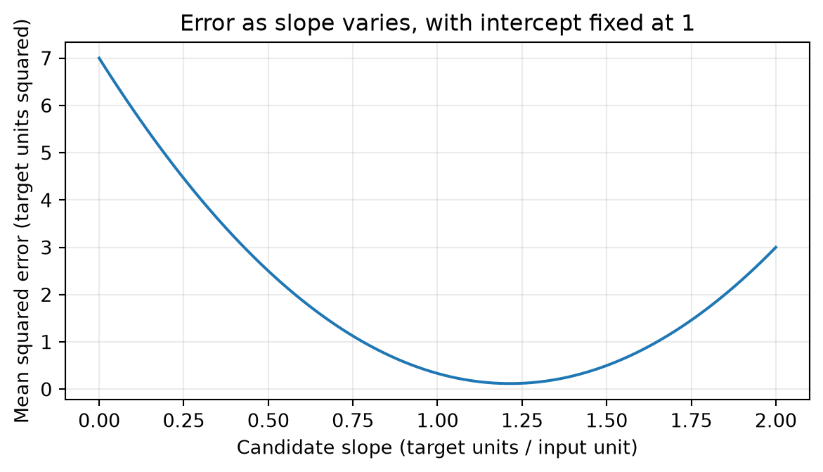
A single error value says how one candidate behaves. A curve shows how error changes across candidates. Hold the intercept at 1 and vary only the slope; this is a one-dimensional slice of a two-parameter problem. It is useful for intuition but does not find the best intercept and slope jointly.
# Step 6: Import plotting tools and evaluate a controlled parameter sweep.import matplotlib.pyplot as plt# Store candidate slopes on an evenly spaced dimensionless teaching grid.slope_candidates = np.linspace(0.0, 2.0, 101)# Keep one error per candidate so the horizontal and vertical values align.candidate_errors = []for slope_value in slope_candidates:# Hold the intercept fixed to isolate the effect of the slope. candidate_predictions = slope_value * input_values + candidate_intercept# Calculate the corresponding training-data MSE. candidate_residuals = observed_targets - candidate_predictions candidate_error = np.mean(candidate_residuals **2) candidate_errors.append(candidate_error)# Step 7: Label the plot with both the changing parameter and the measured quantity.figure, axis = plt.subplots(figsize=(6.2, 3.6))axis.plot(slope_candidates, candidate_errors)axis.set_xlabel("Candidate slope (target units / input unit)")axis.set_ylabel("Mean squared error (target units squared)")axis.set_title("Error as slope varies, with intercept fixed at 1")axis.grid(alpha=0.25)figure.tight_layout()plt.show()
Figure 5.1: A synthetic squared-error objective as slope varies with a fixed intercept. This is a one-dimensional slice, not a joint fit of both parameters.
The curve rises on either side of its lowest region. A grid approximates the best slope within its chosen range and resolution; it is not a proof of an exact optimum. Later chapters derive an optimizer and compare its result with numerical solvers. This plot is a description of three fixed observations, not a validation curve or a generalization claim.
5.8 Pitfalls to recognize early
Equation versus assignment:\(w=w-1\) is not an ordinary real-number equality, but weight = weight - 1 updates a stored program value.
Missing parentheses:a + b / n averages only b; (a + b) / n averages the whole numerator.
Confusing indexes and powers:\(x_i\) selects observation \(i\); \(x^i\) raises a number to a power.
Invalid cancellation:\((a+b)/a\) is \(1+b/a\) when \(a\ne0\), not \(b\). A term can be cancelled only when it is a factor of the whole numerator and denominator.
Unstated domains: division, roots, and logarithms each impose restrictions.
Ignoring scale: MSE in meters squared differs numerically from MSE in centimeters squared by a factor of \(10{,}000\) for the same physical errors.
5.9 Exercises and worked answers
Solve a model equation. If \(\widehat{y}=4x+7\) and the desired prediction is 19, what is \(x\)? Answer: subtract 7 to obtain \(4x=12\), then divide by 4: \(x=3\). Substitution gives \(4(3)+7=19\).
Read a sum. Expand \(\frac{1}{3}\sum_{i=1}^3(2i-1)\). Answer: the terms are 1, 3, and 5, so the average is \(9/3=3\). The index values generate the terms; they are not observations from a dataset.
Compare penalties. Targets are \((1,4)\) and predictions are \((2,2)\). Calculate mean absolute and mean squared error. Answer: residuals are \((-1,2)\). Mean absolute error is \((1+2)/2=1.5\) target units; MSE is \((1+4)/2=2.5\) squared units.
Check a logarithm claim. Is \(\ln(2+3)=\ln2+\ln3\)? Answer: the left side is \(\ln5\), whereas the right side is \(\ln6\). The product identity cannot be used for a sum.
Find a valid inverse. Why must \(f(x)=x^2\) have a restricted domain before its inverse is a function? Answer: positive outputs usually have two preimages. On \(x\geq0\), the inverse selects \(\sqrt{y}\) uniquely for \(y\geq0\).
Handle a negative inequality. Solve \(-3w\leq6\). Answer: divide by \(-3\) and reverse the inequality: \(w\geq-2\). Checking \(w=0\) confirms that it satisfies both versions.
Explain a log objective. A candidate assigns probabilities 0.8 and 0.5 to two independent observed events. Write its negative log-likelihood. Answer:\(L=0.8(0.5)=0.4\), so the objective is \(-\ln0.4=-\ln0.8-\ln0.5\). Independence is needed for this product representation; the logarithm identity alone does not establish it.
5.10 One-page revision summary
Idea
Meaning and check
\(f(x;w,b)=wx+b\)
Input \(x\) changes predictions; fitted parameters determine the rule.
\(\sum_i a_i\)
Add one term per observation; inspect limits and parentheses.
\(\frac{1}{n}\sum_i r_i^2\)
Average squared residuals; units are squared target units.
\(\exp(x)\) and \(\ln x\)
Inverse operations; the real logarithm requires \(x>0\).
\(\ln\prod_i p_i=\sum_i\ln p_i\)
Replaces a positive product by a sum; useful for likelihood.
Rearranging equations
Apply reversible operations and record domain restrictions.
Numerical checks
Use hand examples, units, and tolerance comparisons.
Before reading a new equation, identify its output, inputs, fixed parameters, indices, and domain. Then expand one or two terms and check units. That routine will make the vectors and matrices in Chapter 6 easier to read.