Suppose a model’s error is large. Knowing the error value does not tell us which parameter to change or how a small change would affect it. Calculus supplies that local information. A derivative measures sensitivity to one quantity, and a gradient collects sensitivities to several parameters. These objects will let us replace a blind parameter search with an informed update.
The central question is practical: if a parameter changes slightly, what happens to a prediction and then to its loss? We build from a single-variable slope to the chain rule, partial derivatives, and the squared-error gradient. Second derivatives describe curvature and help explain optimization behavior. Numerical checks connect the symbolic formulas with executable calculations.
Prerequisites: functions, powers, sums, exponentials, and logarithms from Chapter 5; dot products and matrix dimensions from Chapter 6. Probability is useful context but is not needed for the main differentiation examples.
Learning objectives:
Interpret a derivative as an instantaneous rate of change.
Apply elementary differentiation rules with their domain restrictions.
Derive a model-loss derivative using the chain rule.
Assemble partial derivatives into a dimensionally consistent gradient.
Use curvature and finite differences to check, rather than overstate, an argument.
9.2 From a secant slope to a derivative
For a function \(f\), the average rate of change between \(t\) and \(t+h\) is
\[
\frac{f(t+h)-f(t)}{h},\qquad h\ne0.
\]
This is the slope of the line joining two points on the graph, called a secant line. If these slopes approach the same finite limit as \(h\) approaches zero from either side, the derivative exists:
The symbol \(h\to0\) describes a limit, not substituting zero into a fraction. If \(t\) is seconds and \(f(t)\) is meters, \(f'(t)\) has units of meters per second. A derivative’s units are output units divided by input units. For a loss differentiated with respect to a coefficient, the units are loss units divided by that coefficient’s units.
For nonzero \(h\), cancellation is valid. Taking the limit yields \(f'(t)=2t\). At \(t=3\), the tangent slope is 6. A small change of 0.01 predicts an approximate output change \(6(0.01)=0.06\); the exact change is \(3.01^2-3^2=0.0601\). The extra \(0.0001\) is the curvature contribution. The tangent approximation becomes locally accurate as the step shrinks.
A function can be continuous but not differentiable. For \(f(t)=|t|\), the left slope at zero is \(-1\) and the right slope is 1, so there is no single derivative there. This matters for absolute-error losses and some neural network functions. Algorithms may use subgradients or other methods, but an ordinary derivative cannot simply be invented at a corner.
9.3 A small differentiation toolkit
Let \(c\) be a constant and let \(f,g\) be differentiable where used.
Rule
Formula and restriction
Constant
\(\frac{d}{dt}c=0\).
Power
\(\frac{d}{dt}t^k=kt^{k-1}\) on a real domain where the power is differentiable.
Sum and scale
\((af+bg)'=af'+bg'\) for constants \(a,b\).
Product
\((fg)'=f'g+fg'\).
Quotient
\((f/g)'=(f'g-fg')/g^2\) when \(g\ne0\).
Exponential
\(\frac{d}{dt}e^t=e^t\).
Natural log
\(\frac{d}{dt}\ln t=1/t\) for \(t>0\).
For example, \(f(t)=3t^2-4t+7\) has derivative \(6t-4\). Constants remain fixed while taking a derivative; a quantity that depends on \(t\) cannot be treated as constant merely because it has another letter.
The product rule is needed because both factors can change. For \(f(t)=t^2\) and \(g(t)=t+1\), differentiate their expanded product \(t^3+t^2\) to get \(3t^2+2t\). The product rule gives the same answer: \(2t(t+1)+t^2(1)=3t^2+2t\). Multiplying the two derivatives would give \(2t\), which is incorrect.
The log rule requires positive input. If a model uses \(\ln p(t)\), both the outer logarithm’s domain and the dependence of \(p\) on \(t\) matter. The derivative is not simply \(1/t\) unless the logarithm’s actual argument is \(t\). That distinction leads to the chain rule.
9.4 The chain rule follows the computation
If \(u=g(t)\) and \(z=f(u)\), with both functions differentiable, then
The outer derivative is evaluated at the inner function’s current value. The notation resembles cancellation of fractions, but the rule is a theorem about composed functions. It is especially useful because a model’s calculation is naturally a sequence of intermediate quantities.
For \(z=(3t+1)^2\), let \(u=3t+1\). Then \(dz/du=2u\) and \(du/dt=3\). Multiplying gives \(dz/dt=6(3t+1)\). Expanding first gives \(z=9t^2+6t+1\), with derivative \(18t+6\), confirming the result. For a logarithmic example, \(z=\ln(1+t^2)\) has derivative \(2t/(1+t^2)\). Its argument is always positive, so the real formula is valid for every real \(t\).
OpenStax’s chain-rule section develops composition with multiple intermediate paths. The same principle underlies differentiation through a computational graph: multiply rates along a path and add contributions when several paths connect a parameter to the output.
9.4.1 Differentiate a prediction and its loss
For one observation, let \(x\) be a fixed input, \(y\) the observed target, \(w\) a slope, and \(b\) an intercept. Define
Here \(e\) is predicted minus observed, the negative of the observed-minus- predicted residual used elsewhere. Squaring makes the loss identical, but we state the sign convention explicitly before differentiating. The factor \(1/2\) is a convenience that cancels the square’s factor of two; it does not change the minimizer of the unregularized loss.
The dependence follows \(w\to\widehat y\to e\to\ell\). Therefore,
and \(\partial\ell/\partial b=e(1)(1)=\widehat y-y\). The partial derivative notation means varying one parameter while holding the other fixed. With \(x=2,y=5,w=1,b=1\), the prediction is 3, \(e=-2\), and the derivatives are \(-4\) for \(w\) and \(-2\) for \(b\). A sufficiently small positive change in either parameter reduces this observation’s loss because the local derivative is negative. Other observations may exert opposing influences; training combines their contributions.
9.5 Partial derivatives and the gradient
A real-valued function of several parameters can be written \(J(\boldsymbol\beta)\) with \(\boldsymbol\beta\in\mathbb R^d\). The partial derivative \(\partial J/\partial\beta_j\) changes coordinate \(j\) while holding the other \(d-1\) coordinates fixed. The gradient is the column vector of all partial derivatives:
For \(J(a,b)=a^2+3ab+2b^2\), the gradient is \((2a+3b,3a+4b)^\top\). When differentiating with respect to \(a\), \(b\) is held fixed, so the derivative of \(3ab\) is \(3b\), not zero. Partial derivatives are defined and illustrated in OpenStax’s multivariable calculus section.
For a differentiable function and a small displacement \(\Delta\boldsymbol\beta\),
The dot product estimates the change in loss. In Euclidean coordinates, the gradient points in the direction of greatest local increase per unit movement; its negative points toward greatest local decrease. This statement concerns an infinitesimal local comparison under a chosen coordinate scale, not a guarantee that an arbitrarily large step will decrease the loss. Rescaling a parameter changes the geometry and may change appropriate step sizes.
The directional derivative in unit direction \(\mathbf u\) is \(\nabla J^\top\mathbf u\). The unit-length condition makes rates in different directions comparable. See OpenStax on directional derivatives and gradients for the geometric relationship. When parameters have different physical units, a unit Euclidean step in the raw coordinates requires interpretation or an appropriate scaling convention.
9.6 Deriving the mean squared-error gradient
Let \(D\in\mathbb R^{n\times d}\) be a fixed design matrix, including an intercept column if desired. Let \(\boldsymbol\beta\in\mathbb R^d\) be the parameter vector and \(\mathbf y\in\mathbb R^n\) the target vector. Write the prediction for observation \(i\) as \(\widehat y_i=\sum_{j=1}^d D_{ij}\beta_j\). The objective is
For one coordinate \(k\), the derivative of the prediction with respect to \(\beta_k\) is \(D_{ik}\). Terms involving other parameters are constant in this partial derivative. Applying the square rule and chain rule gives
The dimensions are \(D\boldsymbol\beta-\mathbf y\in\mathbb R^n\), \(D^\top\in\mathbb R^{d\times n}\), and gradient in \(\mathbb R^d\). The matrix formula is a compact collection of the scalar sums, not a different algorithm. If the objective were half the MSE, the leading 2 would disappear. Loss and gradient must use the same convention.
9.6.1 Implement and inspect the scalar contributions
Make a tiny intercept-plus-one-feature design matrix.
Write a scalar-returning MSE function with explicit shape checks.
Accumulate each gradient coordinate with ordinary loops.
Verify the same result with the matrix formula and a hand calculation.
# Step 1: Import NumPy and define the complete data state for this chapter.import numpy as np# Each row is one artificial observation; the first column multiplies the intercept.design_matrix = np.array([[1.0, 0.0], [1.0, 1.0], [1.0, 2.0]])# Targets are dimensionless teaching values in the same observation order.observed_targets = np.array([1.0, 2.0, 2.0])# Parameters are ordered as intercept followed by slope.candidate_coefficients = np.array([0.5, 1.0])# Step 2: Represent precisely the MSE objective that our derivatives describe.def mean_squared_error(coefficients, features_with_intercept, targets):"""Return scalar MSE for a coefficient vector and paired observations. coefficients has shape (d,), features_with_intercept has shape (n, d), and targets has shape (n,). Inputs must be finite real teaching data. The returned quantity is in squared target units. """# Matrix multiplication yields exactly one prediction per observation. predictions = features_with_intercept @ coefficients# Matching one-dimensional shapes prevent accidental two-dimensional broadcasting.if predictions.shape != targets.shape:raiseValueError("Targets and predictions must have identical shapes.")# Use predicted-minus-observed errors consistently with the derivative. prediction_errors = predictions - targetsreturnfloat(np.mean(prediction_errors **2))# Step 3: Map each partial derivative's summation directly into loops.def explicit_mse_gradient(coefficients, features_with_intercept, targets):"""Return the MSE gradient, shape (d,), using explicit scalar sums. Inputs follow mean_squared_error. Each returned entry differentiates squared target units with respect to the corresponding coefficient unit. """# Store the observation count for the mean-loss normalization. number_of_observations =len(targets)# Allocate one derivative for each coefficient. gradient = np.zeros(len(coefficients))# Compute each row's prediction once before accumulating coordinate contributions. predictions = features_with_intercept @ coefficientsfor coefficient_index inrange(len(coefficients)):# Reset the derivative sum for this coordinate. derivative_total =0.0for observation_index inrange(number_of_observations):# Error for this row determines its direction of pressure on the coefficient. prediction_error = predictions[observation_index] - targets[observation_index]# The design entry is the prediction's derivative with respect to this coefficient. feature_value = features_with_intercept[observation_index, coefficient_index] derivative_total = derivative_total +2.0* prediction_error * feature_value gradient[coefficient_index] = derivative_total / number_of_observationsreturn gradient# Step 4: Check the scalar derivation against its matrix form and a hand result.# The three errors at this candidate are (-0.5, -0.5, 0.5).prediction_errors = design_matrix @ candidate_coefficients - observed_targets# This is the compact expression derived in the text, with shape (2,).matrix_gradient =2.0* design_matrix.T @ prediction_errors /len(observed_targets)# Obtain the same two derivatives by explicit summation.loop_gradient = explicit_mse_gradient(candidate_coefficients, design_matrix, observed_targets)assert np.allclose(loop_gradient, [-1.0/3.0, 1.0/3.0])assert np.allclose(loop_gradient, matrix_gradient)print("Candidate MSE:", mean_squared_error(candidate_coefficients, design_matrix, observed_targets))print("Gradient, intercept then slope:", loop_gradient)
Candidate MSE: 0.25
Gradient, intercept then slope: [-0.33333333  0.33333333]
The intercept derivative is negative and the slope derivative is positive at this candidate. They need not share a sign even though both influence every prediction. In the next chapter, a gradient-descent update will subtract a small multiple of these derivatives from their respective parameters.
9.7 Second derivatives, the Hessian, and stationary points
The second derivative \(f''(t)\) describes how the first derivative changes. For \(f(t)=(t-3)^2\), \(f''(t)=2\): its slope increases at a constant rate. For a twice differentiable function of several parameters, the Hessian\(H\in\mathbb R^{d\times d}\) has entries \(H_{jk}=\partial^2J/(\partial\beta_j\partial\beta_k)\). With continuous second partial derivatives, mixed derivatives agree and the Hessian is symmetric.
Differentiate the MSE gradient once more:
\[
H=\frac2nD^\top D.
\]
It does not depend on \(\boldsymbol\beta\) because MSE for a linear model is quadratic in its parameters. For any vector \(\mathbf v\), \(\mathbf v^\top H\mathbf v=(2/n)\|D\mathbf v\|_2^2\geq0\). Thus the Hessian is positive semidefinite. If \(D\) has full column rank, the expression is strictly positive for nonzero \(\mathbf v\), giving positive definiteness and a unique least-squares minimizer. Redundant columns permit flat directions instead.
A stationary point has zero gradient. For a differentiable function at an interior local minimum, the gradient must be zero. The converse is false. For \(f(t)=t^3\), the derivative is zero at zero, but the function keeps increasing through that point. For \(J(a,b)=a^2-b^2\), the origin is a saddle: the function rises in one direction and falls in another. A constrained minimum can also occur on a boundary where the ordinary gradient is nonzero. These conditions must be checked before interpreting “the derivative is zero” as “the optimization problem is solved.”
If a function is twice continuously differentiable near the current point, a second-order local approximation is
For a quadratic this expression is exact; for a general smooth function it omits higher-order effects. Curvature explains why a step suggested by a local slope can overshoot when the step is too large.
9.8 Finite differences as a gradient check
A computer can approximate a derivative by evaluating nearby function values. The central difference for coordinate \(j\) is
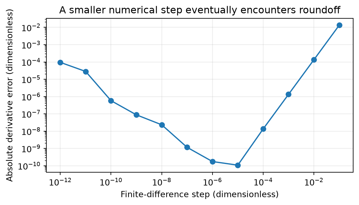
where \(\mathbf e_j\) is a unit vector with one in position \(j\) and zero elsewhere. Under sufficient smoothness, the truncation error is order \(h^2\) for a scalar coordinate step. But very small \(h\) subtracts nearly equal floating-point values and can amplify roundoff. Smaller is not always better. The step should also be interpreted relative to the parameter’s scale.
# Step 5: Compare each analytic derivative with an independent numerical calculation.def central_difference_gradient(coefficients, features_with_intercept, targets, step_size):"""Approximate the MSE gradient by central differences in each coordinate. Shapes follow mean_squared_error. step_size is a positive coordinate step in the dimensionless teaching parameterization. Returns an array of shape (d,). This is a diagnostic for small problems, not a production training method. """if step_size <=0.0:raiseValueError("The finite-difference step must be positive.")# Store one independent approximation per coefficient. numerical_gradient = np.zeros(len(coefficients))for coefficient_index inrange(len(coefficients)):# Copies prevent a diagnostic perturbation from changing the caller's coefficients. plus_coefficients = coefficients.copy() minus_coefficients = coefficients.copy()# Perturb only the coordinate whose partial derivative is being checked. plus_coefficients[coefficient_index] += step_size minus_coefficients[coefficient_index] -= step_size# Re-evaluate the full objective on both sides of the original candidate. plus_loss = mean_squared_error(plus_coefficients, features_with_intercept, targets) minus_loss = mean_squared_error(minus_coefficients, features_with_intercept, targets) numerical_gradient[coefficient_index] = (plus_loss - minus_loss) / (2.0* step_size)return numerical_gradient# A moderate step is small relative to the order-one teaching parameters.finite_difference_step =1e-6# The numerical estimate depends only on objective values, not the gradient formula.numerical_gradient = central_difference_gradient( candidate_coefficients, design_matrix, observed_targets, finite_difference_step)assert np.allclose(numerical_gradient, loop_gradient, atol=1e-8, rtol=1e-7)print("Finite-difference gradient:", numerical_gradient)# Step 6: Inspect curvature through the Hessian's eigenvalues.# eigvalsh is designed for real symmetric matrices and returns their eigenvalues.mse_hessian =2.0* design_matrix.T @ design_matrix /len(observed_targets)hessian_eigenvalues = np.linalg.eigvalsh(mse_hessian)assert np.all(hessian_eigenvalues >0.0)print("MSE Hessian eigenvalues:", hessian_eigenvalues)
Agreement at one point is useful evidence but cannot prove a gradient formula for every input. Check a few nontrivial candidates and independently derived special cases. Avoid nondifferentiable points when checking an ordinary derivative. A numerical comparison can also miss a shared bug if the analytic and numerical paths reuse an incorrect objective definition, so first confirm that the objective itself represents the intended mathematics.
9.8.1 A controlled step-size experiment
We now approximate the derivative of \(f(t)=e^t+t^3\) at \(t=0.7\) using several \(h\) values. Its analytic derivative is \(e^t+3t^2\). The function, evaluation point, and number format remain fixed; only the step changes.
# Step 7: Measure how finite-difference error depends on the step size.import matplotlib.pyplot as plt# Fix the evaluation point away from any domain boundary.evaluation_point =0.7# The exact analytic expression provides the comparison value.analytic_derivative = np.exp(evaluation_point) +3.0* evaluation_point **2# Sweep from a coarse step toward a step where subtraction roundoff can matter.step_sizes = np.logspace(-1, -12, 12)# Store one absolute error for each step, in matching order.derivative_errors = []for step_size in step_sizes:# Evaluate the function on either side without using its derivative formula. plus_value = np.exp(evaluation_point + step_size) + (evaluation_point + step_size) **3 minus_value = np.exp(evaluation_point - step_size) + (evaluation_point - step_size) **3# The central difference estimates the local rate of change. derivative_estimate = (plus_value - minus_value) / (2.0* step_size)# Compare against the independently differentiated expression. absolute_error =abs(derivative_estimate - analytic_derivative) derivative_errors.append(absolute_error)# Step 8: Logarithmic axes expose changes over several orders of magnitude.figure, axis = plt.subplots(figsize=(6.2, 3.6))axis.loglog(step_sizes, derivative_errors, marker="o")axis.set_xlabel("Finite-difference step (dimensionless)")axis.set_ylabel("Absolute derivative error (dimensionless)")axis.set_title("A smaller numerical step eventually encounters roundoff")axis.grid(alpha=0.25)figure.tight_layout()plt.show()
Figure 9.1: Central-difference error for a fixed smooth teaching function. Very small steps amplify floating-point cancellation.
The errors balance approximation and roundoff effects; the best numerical step depends on the function, evaluation point, scale, and number format. This example motivates a range of diagnostic step sizes, rather than a rule to use the smallest representable perturbation.
9.9 Exercises and worked answers
Differentiate a polynomial. Find the derivative of \(2t^3-5t+4\). Answer:\(6t^2-5\). The constant contributes zero.
Use the chain rule. Differentiate \(\ln(2+t^2)\). Answer:\(2t/(2+t^2)\). The outer derivative contributes \(1/(2+t^2)\) and the inner derivative contributes \(2t\); the domain is all real \(t\) because the log argument is positive.
Read units. If loss is in meters squared and a parameter is in meters per second, what units does its derivative have? Answer:\((\text{meters}^2)/(\text{meters/second})\), or meter-seconds. A parameter-update step must account for these units and its scaling convention.
Find partial derivatives. For \(J(a,b)=a^2+ab+3b^2\), find the gradient. Answer:\((2a+b,a+6b)^\top\), holding the other coordinate fixed in each partial derivative.
Identify a saddle. Is the stationary origin of \(a^2-b^2\) a minimum? Answer: no. Along \((a,0)\) the loss is positive away from zero; along \((0,b)\) it is negative. The directions disagree about increase versus decrease.
Check a loss normalization. If \(J\) is MSE and \(K=J/2\), what happens to the gradient and minimizer? Answer:\(\nabla K=\nabla J/2\). The minimizer is unchanged, but the same numerical learning rate yields a smaller update for \(K\).
Interpret numerical disagreement. A gradient check worsens when \(h\) decreases from \(10^{-6}\) to \(10^{-14}\). Must the formula be wrong? Answer: no. Floating-point cancellation can dominate at tiny steps. Compare multiple moderate steps, parameter scales, and hand-derived cases.
9.10 One-page revision summary
Tool
Role in learning
Derivative
Local sensitivity to one input or parameter; check units.
Chain rule
Follow the dependence from parameter to prediction to loss.
Partial derivative
Change one coordinate, holding the others fixed.
Gradient
Vector of partial derivatives, with the parameter vector’s dimension.
MSE gradient
\((2/n)D^\top(D\boldsymbol\beta-\mathbf y)\).
Hessian
Matrix of second derivatives; describes local curvature.
Stationary point
Zero gradient; more information is needed to classify it.
Finite difference
Independent numerical check with truncation/roundoff tradeoffs.
Derive the loss and derivative together, check dimensions, and test a tiny example before training. Chapter 10 uses this local information to construct a complete numerical fitting procedure.