The useful question about a predictive model is how it behaves on the observations it will encounter later. A low error on data used for fitting does not answer that question: the model has already had an opportunity to adapt to those data. A defensible experiment therefore separates learning, choosing, and final assessment.
12.1 Learning objectives and prerequisites
After this chapter, you should be able to distinguish fitting loss from reporting metrics, construct training/validation/test partitions, select a split appropriate for groups or time, compare with a baseline, interpret overfitting and learning curves, and tune a small set of hyperparameters without consulting the final test set. You should recognize both direct target leakage and indirect leakage through preprocessing or repeated model selection.
Prerequisites are elementary statistics and the task definition and exploration in Chapter 11. We introduce a library regression model as an experimental object. Its mathematics and explicit implementation come later in Chapter 14. A pipeline will first appear as an ordered sequence of operations; Chapter 13 explains its mechanics in detail. You can understand the evaluation procedure before understanding how the model solves its fitting problem.
12.2 Generalization is a question about a population
Let \(\mathbf{x}_i\in\mathbb{R}^{p}\) contain \(p\) features for observation \(i\), let \(y_i\) be its target, and let \(\hat{f}\) be a fitted prediction function. Its prediction is \(\hat{y}_i=\hat{f}(\mathbf{x}_i)\). Generalization is the model’s behavior on new observations from the intended application. It always refers to a population and a setting: unseen trials from known people, unseen people, future days, and new devices are different settings.
For a loss function \(\ell\), the population prediction risk is
\(P\) denotes the intended distribution of feature/target pairs, and the expectation averages over new pairs from that distribution. We usually cannot calculate this quantity exactly. Instead, we use an evaluation set of \(m\) observations:
This is an estimate, not a guarantee. Its usefulness depends on how evaluation observations were collected and whether development choices used them. A clean split from the wrong population still answers the wrong question. More test rows from a few correlated people also do not provide the same evidence as more independently sampled people.
12.3 Loss functions and evaluation metrics
A training loss is the quantity optimized while fitting parameters. A metric is a quantity used to assess predictions. They can be the same mathematical function used on different data, or different functions chosen for different purposes. A training objective may also include a regularization penalty that is not itself a prediction error metric.
For regression, define the prediction error \(e_i=\hat{y}_i-y_i\). Three common metrics are
MAE is the mean absolute error, MSE the mean squared error, and RMSE the root mean squared error. Lower values are better. If speed is measured in m/s, MAE and RMSE have units m/s, while MSE has squared units. Squaring gives unusually large errors extra influence. MAE gives equal additional penalty for each additional unit of absolute error. Which behavior is appropriate depends on the prediction goal and costs of mistakes.
For example, errors \([0.1,-0.2,0.3]\) m/s have MAE \(0.6/3=0.2\) m/s and MSE \((0.01+0.04+0.09)/3\approx0.0467\)\((\text{m/s})^2\). RMSE is approximately \(0.216\) m/s. Averaging signed errors would give approximately \(0.067\) m/s and would hide cancellation between overprediction and underprediction.
For a nonconstant evaluation target, \(R^2=1\) means perfect predictions; \(R^2=0\) matches the sum of squared errors of the evaluation-set mean; and negative values are possible. The evaluation mean is part of this metric’s definition, not a permissible way to fit a baseline. Constant targets make the displayed ratio undefined, and library handling requires care. Do not interpret \(R^2\) as an error in physical units.
For classification, first define the positive class. A true positive (TP) is a correctly predicted positive; a false positive (FP) is a negative predicted positive; a false negative (FN) is a positive predicted negative; a true negative (TN) is a correctly predicted negative. Then
Precision asks what fraction of positive predictions are correct. Recall asks what fraction of actual positives are found. Their harmonic mean is \(F_1=2TP/(2TP+FP+FN)\) when the denominator is nonzero. If only two of 100 cases are positive, predicting negative for everyone gives 98% accuracy and zero recall. Report class counts and the relevant mistakes rather than accuracy alone. Undefined denominators need an explicit reporting convention. Metrics for probability predictions, threshold selection, and ranking receive fuller treatment with classification; choose their rules using development data. The official scoring guide provides definitions and task-based selection guidance.
12.3.1 Step 1: Connect formulas to numerical code
The following tiny calculation is independent of any fitted model. It compares an explicit calculation with the corresponding library functions.
# Step 1: Calculate regression metrics directly from three predictions.import numpy as npimport pandas as pdimport matplotlib.pyplot as pltfrom sklearn.metrics import mean_absolute_error, root_mean_squared_error# Measured reference speeds for three hypothetical observations, in m/s.actual_speeds = np.array([1.0, 1.4, 1.2])# Predicted speeds, with known positive and negative prediction errors.predicted_speeds = np.array([1.1, 1.2, 1.5])# Subtract measured values to obtain signed errors in m/s.prediction_errors = predicted_speeds - actual_speeds# Absolute errors prevent overprediction and underprediction from canceling.manual_mae = np.mean(np.abs(prediction_errors))# Squared errors emphasize larger mistakes before averaging.manual_mse = np.mean(prediction_errors **2)# Restore the target's units by taking the square root.manual_rmse = np.sqrt(manual_mse)# Check that explicit formulas and library definitions agree.assert np.isclose(manual_mae, mean_absolute_error(actual_speeds, predicted_speeds))assert np.isclose( manual_rmse, root_mean_squared_error(actual_speeds, predicted_speeds))print("MAE (m/s):", round(manual_mae, 3))print("MSE ((m/s)^2):", round(manual_mse, 4))print("RMSE (m/s):", round(manual_rmse, 3))
MAE (m/s): 0.2
MSE ((m/s)^2): 0.0467
RMSE (m/s): 0.216
12.4 Separate fitting, choosing, and final assessment
The training set fits model parameters, such as regression coefficients. The validation set assesses development choices, such as which features or polynomial degree to use. The test set provides a final assessment after choices are fixed. Hyperparameters are settings chosen outside an individual parameter-fitting operation. Their names differ by algorithm; polynomial degree, regularization strength, and tree depth are examples.
One simple procedure is:
Define the task, metric, baseline, and split rules.
Reserve a test set using those rules.
Divide remaining development data into training and validation portions.
Fit each candidate on training data and compare on validation data.
Fix the chosen procedure and refit it on all development data.
Evaluate on the final test set and document the result and limitations.
Refitting on all development data is appropriate because the test set remains separate. If the test result is disappointing, investigate and document it. Continuing to choose models until that same test score improves turns the test set into another validation set. A fresh independent evaluation or a revised reporting claim is then needed. The cross-validation guide explains the roles of validation and held-out assessment.
There is no universally correct split percentage. Small datasets may make a single validation estimate unstable; large test fractions reduce data available for fitting. Rare classes, the number of groups, and forecast horizons can matter more than a percentage. A reproducible random seed makes a particular partition repeatable; it does not prove that partition is representative.
12.4.1 Match the split to the application
Intended prediction
Suitable starting split
Principal concern
New independent rows from the same collection process
Random holdout; shuffled folds within development
Hidden dependence or collection shift
New people, devices, sites, or recording sessions
Group-disjoint holdout and group-aware development folds
Choosing the right grouping level
Future observations using past information
Chronological holdout and forward-in-time validation
Future information and overlapping horizons
Class labels with scarce positive examples
Stratification when compatible with dependence constraints
Enough examples and groups per class
Stratification approximately preserves class proportions; it does not remove dependence. Randomly splitting overlapping recording windows is especially problematic because shared raw samples can cross the boundary. For new-person predictions, group all of each person’s sessions together. If both new-person generalization and future prediction are requirements, design a split that enforces both; a convenient random splitter does not supply that protocol automatically.
12.4.2 Step 2: Check grouped and chronological boundaries
These are split demonstrations, not experiments estimating performance. Group identifiers remain metadata. The time example assumes equally spaced observations in chronological order. gap=1 deliberately leaves one unused row between training and validation; real gaps must follow the forecast horizon, feature lookback, and label availability. The TimeSeriesSplit documentation describes its expanding training sets and equally spaced data assumption for comparable fold durations.
# Step 2: Verify that split boundaries match groups and time.from sklearn.model_selection import GroupKFold, TimeSeriesSplit# Twelve rows come from four simulated people, three rows per person.group_identifiers = np.repeat(np.arange(4), 3)# Store an arbitrary one-column feature matrix for demonstrating indices.grouped_features = np.arange(12).reshape(-1, 1)# Hold out one person's rows per fold in this four-group example.grouped_folds = GroupKFold(n_splits=4)for fold_number, (training_rows, validation_rows) inenumerate( grouped_folds.split(grouped_features, groups=group_identifiers), start=1):# Convert row-level IDs into sets of people for this fold. training_people =set(group_identifiers[training_rows])# Store the people excluded from fitting in this fold. validation_people =set(group_identifiers[validation_rows])assert training_people.isdisjoint(validation_people)print("Group fold", fold_number, "validation people:", sorted(validation_people))# Eighteen equally spaced rows are already sorted from past to future.ordered_features = np.arange(18).reshape(-1, 1)# Use three validation blocks, each three observations long, with a one-row gap.temporal_folds = TimeSeriesSplit(n_splits=3, test_size=3, gap=1)for fold_number, (training_rows, validation_rows) inenumerate( temporal_folds.split(ordered_features), start=1):assert training_rows.max() < validation_rows.min()assert validation_rows.min() - training_rows.max() ==2print("Time fold", fold_number,"last training row:", training_rows.max(),"first validation row:", validation_rows.min() )
Group fold 1 validation people: [np.int64(3)]
Group fold 2 validation people: [np.int64(2)]
Group fold 3 validation people: [np.int64(1)]
Group fold 4 validation people: [np.int64(0)]
Time fold 1 last training row: 7 first validation row: 9
Time fold 2 last training row: 10 first validation row: 12
Time fold 3 last training row: 13 first validation row: 15
12.5 Underfitting, overfitting, and regularization
An underfitting model misses important structure, giving poor training and validation performance. A straight line fitted to a pronounced curve is a possible example. An overfitting model adapts to details of the training sample that do not transfer, often giving a much lower training error than validation error. A training-validation gap is a diagnostic clue, not a proof: population differences, leakage, or an implementation mistake may also cause a gap.
The bias-variance intuition describes two sources of estimation difficulty. A restrictive procedure can repeatedly miss a real pattern, producing systematic error often associated with bias. A flexible procedure can change substantially when the training sample changes, producing variability often associated with variance. This is a qualitative introduction; it does not claim that every algorithm obeys a simple monotonic tradeoff in every setting. Irreducible uncertainty from unobserved variables or measurement noise can remain even with a well-chosen model.
Regularization restricts or discourages certain fitted solutions. For example, a squared-coefficient penalty gives an objective of the form
Here \(n\) counts training observations, \(w_j\) is a model coefficient, and \(\lambda\ge0\) controls the penalty strength under this stated scaling convention. The intercept is typically treated separately in this formulation. Larger \(\lambda\) discourages large coefficients more strongly and may reduce sensitivity to the sample while making the fit less flexible. Feature units matter because changing units changes coefficient sizes. Exact conventions and solvers are introduced with the relevant model. Regularization is not a remedy for an invalid split or a leaked feature.
12.6 A complete development experiment with cross-validation
Cross-validation (CV) repeats the training-validation operation within development data. In \(K\)-fold CV, each of \(K\) blocks serves once as validation while the other blocks fit a fresh model. The average fold error summarizes that candidate’s validation behavior under this scheme. Overlapping training sets make fold scores dependent, so their standard deviation is descriptive variability, not automatically a confidence interval.
This experiment creates 240 independent synthetic pairs. A dimensionless feature influences a continuous target in m/s through a quadratic expression. We compare polynomial degrees 1, 2, and 12, with a constant-mean baseline. PolynomialFeatures creates powers of the input, and LinearRegression fits coefficients to those columns. The degree is a hyperparameter; the fitted coefficients are parameters. All steps are placed in a pipeline so later learned preparation can be repeated within folds.
This is a small demonstration, not a benchmark or a physiology model. Its question is whether the validation procedure distinguishes useful curvature from extra flexibility on this constructed dataset.
12.6.1 Step 3: Generate data and reserve the final test
# Step 3: Prepare independent synthetic regression pairs and a sealed test set.from sklearn.dummy import DummyRegressorfrom sklearn.linear_model import LinearRegressionfrom sklearn.model_selection import train_test_split, KFold, GridSearchCVfrom sklearn.model_selection import cross_val_score, learning_curvefrom sklearn.pipeline import Pipelinefrom sklearn.preprocessing import PolynomialFeatures# Fix the generator for repeatable synthetic pairs.regression_generator = np.random.default_rng(7)# Store 240 dimensionless feature values as a samples-by-features matrix.regression_features = regression_generator.uniform(-2.0, 2.0, size=(240, 1))# Extract the only feature as a one-dimensional array for target construction.feature_values = regression_features[:, 0]# Simulate target noise in m/s without giving it to the predictor.target_noise = regression_generator.normal(0.0, 0.08, size=240)# Construct a curved target relationship in m/s for the teaching experiment.regression_targets =0.8+0.15* feature_values +0.18* feature_values **2regression_targets = regression_targets + target_noise# Return features and targets in matching development/test partitions.# The final 25% holdout is not used for selecting a polynomial degree.development_features, final_test_features, development_targets, final_test_targets = ( train_test_split( regression_features, regression_targets, test_size=0.25, random_state=42 ))# Use the same five development folds for every candidate and baseline.development_folds = KFold(n_splits=5, shuffle=True, random_state=42)assert development_features.shape == (180, 1)assert final_test_features.shape == (60, 1)print("Development and test shapes:", development_features.shape, final_test_features.shape)
Development and test shapes: (180, 1) (60, 1)
Random splitting is appropriate here because the pairs were generated independently for this example. It is not a replacement for the group or temporal procedures above. During real development, record seeds, indices or stable record IDs, package versions, and the full candidate set so the experiment can be reproduced.
12.6.2 Step 4: Compare a baseline and choose a degree within development data
A baseline is a simple reference procedure. For squared-error regression, a training-target mean is a natural constant predictor. It must learn that constant separately in each training fold. A baseline that uses the complete dataset mean has already used validation or test targets. The DummyRegressor API supplies an explicit strategy="mean" for this comparison.
scikit-learn scoring functions used in search follow a larger-is-better convention. Therefore neg_root_mean_squared_error returns negative RMSE: \(-0.08\) is better than \(-0.20\). Negating those scores for reporting restores familiar positive errors. GridSearchCV fits every listed degree on every fold, compares the mean validation score, and, with refit=True, fits the chosen pipeline on all development data. See the search API.
# Step 4: Establish a baseline and select model complexity using development CV.# Predict the mean of the targets available in each fitting operation.constant_baseline = DummyRegressor(strategy="mean")# Compute five held-out fold scores without touching the final test.baseline_negative_scores = cross_val_score( constant_baseline, development_features, development_targets, cv=development_folds, scoring="neg_root_mean_squared_error")# Restore positive RMSE for a readable comparison in target units.baseline_cv_rmse =-baseline_negative_scores.mean()# Apply feature expansion before coefficient fitting in each fold.# include_bias=False avoids adding a second constant beside the fitted intercept.candidate_pipeline = Pipeline([ ("polynomial", PolynomialFeatures(include_bias=False)), ("regression", LinearRegression(fit_intercept=True)),])# Specify the complete, small candidate set before examining the test set.candidate_settings = {"polynomial__degree": [1, 2, 12]}# Request training scores too, so the training-validation gap can be inspected.degree_search = GridSearchCV( candidate_pipeline, candidate_settings, cv=development_folds, scoring="neg_root_mean_squared_error", refit=True, return_train_score=True, error_score="raise", n_jobs=1)degree_search.fit(development_features, development_targets)# Convert search output into a compact comparison table.search_results = pd.DataFrame(degree_search.cv_results_)# Keep the degree and restore positive errors in m/s for both score columns.comparison_table = pd.DataFrame({"degree": search_results["param_polynomial__degree"],"training_RMSE_m_per_s": -search_results["mean_train_score"],"validation_RMSE_m_per_s": -search_results["mean_test_score"],})print("Baseline mean CV RMSE (m/s):", round(baseline_cv_rmse, 3))print(comparison_table.round(4).to_string(index=False))print("Selected settings:", degree_search.best_params_)
The mean_test_score column in this search object refers to the held-out CV folds inside the development set. Its library name does not mean that the final test set was used. This distinction prevents a common misunderstanding when reading search output.
The degree with the lowest validation RMSE is selected under this protocol. Compare its gap and baseline error before drawing a conclusion. The known quadratic generator explains why degree 2 is a sensible candidate, but selection still uses measured development performance. A higher degree can reduce training error while adding unstable behavior, particularly near or beyond the observed feature range. CV assesses the listed candidates; it does not demonstrate that the selected model is best among all possible models.
Because we select using the fold scores, the winning CV score can be optimistic about the whole selection process. The untouched test set supplies the final assessment here. Nested cross-validation is an alternative when estimating selection procedures through outer held-out folds; it costs more fits and is beyond this first example. Large, repeatedly adapted searches need special care even when every individual fit is technically inside a fold.
The checked run selects degree 2. Mean validation RMSE values are 0.2130, 0.0764, and 0.0777 m/s for degrees 1, 2, and 12, respectively, compared with 0.271 m/s for the constant baseline. Degree 12 lowers mean training RMSE from 0.0759 to 0.0737 m/s relative to degree 2 while slightly worsening validation RMSE. That is a small instance of extra flexibility improving the fit without improving the held-out development comparison.
12.7 Learning curves: decide what additional data might help
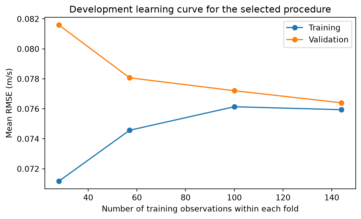
A learning curve varies the number of training observations and compares training and validation errors while holding the model procedure fixed. It addresses a different question from a validation curve, which varies a hyperparameter. Very small training sets can give optimistic training errors and noisy validation results. With more data, a narrowing gap can suggest reduced sample sensitivity. Persistently high errors on both sides can suggest missing features, an unsuitable model, or substantial noise.
These are diagnostic patterns, not automatic prescriptions. More data from the same narrow population may not solve deployment shift. A curve that has flattened over a short range may change later. The learning-curve guide explains their role in examining bias and variance behavior.
12.7.1 Step 5: Plot curves using development folds only
# Step 5: Inspect data-size sensitivity without consulting the final test set.# Keep the model degree selected by development CV fixed for this diagnostic.selected_pipeline = degree_search.best_estimator_# Fit fresh copies at four fractions of each fold's available training rows.training_sizes, negative_training_scores, negative_validation_scores = learning_curve( selected_pipeline, development_features, development_targets, cv=development_folds, train_sizes=[0.2, 0.4, 0.7, 1.0], scoring="neg_root_mean_squared_error", shuffle=True, random_state=42, n_jobs=1, error_score="raise")# Average across folds separately for each training-set size.mean_training_errors =-negative_training_scores.mean(axis=1)# Store mean held-out fold errors in m/s for the second curve.mean_validation_errors =-negative_validation_scores.mean(axis=1)# Allocate a figure with axes that identify data quantity and error units.figure, axis = plt.subplots(figsize=(6.5, 4))axis.plot(training_sizes, mean_training_errors, marker="o", label="Training")axis.plot(training_sizes, mean_validation_errors, marker="o", label="Validation")axis.set_xlabel("Number of training observations within each fold")axis.set_ylabel("Mean RMSE (m/s)")axis.set_title("Development learning curve for the selected procedure")axis.legend()figure.tight_layout()plt.show()assert np.isfinite(mean_training_errors).all()assert np.isfinite(mean_validation_errors).all()
Figure 12.1: Mean training and held-out validation RMSE across five development folds at four training sizes. The final test set contributes to neither curve.
Every plotted value comes from development data. This curve is exploratory because the degree was already selected using these folds. It is not an independent generalization estimate, and the smooth connecting lines do not represent measured intermediate training sizes. Inspect both curves and the underlying fold variability before deciding to collect data or change a model.
12.7.2 Step 6: Evaluate the fixed procedure at the end
The model procedure, metric, and baseline have now been fixed. Evaluate the selected pipeline and the predetermined baseline on the same final test rows. The baseline is fitted on development targets only. This is one final comparison, not another search. Do not use its results to choose another degree within this experiment.
# Step 6: Produce the final, prespecified comparison on unseen synthetic pairs.# Fit the constant baseline using all development targets and no test targets.constant_baseline.fit(development_features, development_targets)# The selected pipeline was already refitted on all development data by search.final_predictions = selected_pipeline.predict(final_test_features)# Obtain the baseline's predictions for the identical test observations.final_baseline_predictions = constant_baseline.predict(final_test_features)# Measure the selected model's RMSE in the target's original units.final_model_rmse = root_mean_squared_error(final_test_targets, final_predictions)# Measure the baseline under the same metric and split.final_baseline_rmse = root_mean_squared_error( final_test_targets, final_baseline_predictions)# Add MAE as a prespecified descriptive companion in the same physical units.final_model_mae = mean_absolute_error(final_test_targets, final_predictions)print("Final model RMSE (m/s):", round(final_model_rmse, 3))print("Final baseline RMSE (m/s):", round(final_baseline_rmse, 3))print("Final model MAE (m/s):", round(final_model_mae, 3))assert final_predictions.shape == final_test_targets.shapeassert np.isfinite(final_predictions).all()
Final model RMSE (m/s): 0.074
Final baseline RMSE (m/s): 0.303
Final model MAE (m/s): 0.059
These printed numbers summarize one seeded synthetic experiment with a 60-row test set. They do not establish a real sensing accuracy, a clinical result, or a universal ranking of polynomial degrees. The valid conclusion is about this fixed procedure under this constructed distribution. A broader study would also consider uncertainty, independent collection, subgroup behavior, and whether its error meets a requirement established by the application.
For this checked run, final model RMSE is 0.074 m/s and MAE is 0.059 m/s; baseline RMSE is 0.303 m/s. These are rounded execution results, not values to assume for another random sample or another target generator.
12.8 Recognize leakage and evaluation failures
Target leakage occurs when inputs contain information that would not be available when the prediction is made, such as a feature derived from the target or a later outcome. Split leakage includes records or correlated raw information crossing a boundary intended to represent new people or times. Preprocessing leakage occurs when validation/test values help fit means, imputers, encoders, feature selectors, or other preparation used to assess a model. The next chapter prevents the last category with training-fold pipelines.
Some failures are subtler. Trying 100 manual feature sets against one validation set is a search even without a search API. Choosing the easiest random seed after seeing scores is another selection step. Rebalancing or augmenting the complete dataset before splitting can place related examples across the boundary. A model can also learn a site or device shortcut that is predictive in the table but fails where the collection process changes. Keep a record of development decisions and align every operation with the prediction timing and split unit.
Computationally, CV repeats fitting. If \(H\) candidates each use \(K\) folds, a simple exhaustive search performs \(HK\) fold fits plus a final refit when requested. Learning curves add roughly one fit per fold and training size. The tiny candidate set here keeps that cost practical. Memory and time of each fit depend on the underlying model and expanded feature count. Do not launch a large search merely because the API makes it one line.
12.9 Exercises and worked answers
Choose a metric. A predictor estimates trial speed. You want errors in m/s and additional sensitivity to occasional large mistakes. Which metric is a starting choice?
Answer: RMSE has m/s units and squares errors before averaging, emphasizing large errors. Also inspect MAE and individual error patterns. An application with asymmetric costs may require a different loss or additional reporting.
Explain a baseline. Why is the mean of all targets an invalid baseline for a held-out test?
Answer: It uses test labels to fit the predictor. Fit the mean on the training portion of each development fold, then on all development data for the final comparison. For MAE, a training median is an appropriate alternative constant baseline.
Spot test reuse. After final evaluation, degree 12 is tried because the test error looked high. Can the better test score be reported as an untouched assessment?
Answer: No. The test result influenced a development choice. Record the reuse and obtain independent evaluation for an unchanged final procedure, or describe the result as exploratory rather than untouched testing.
Count fits. A grid contains four settings and uses five folds with a final refit. How many fits are performed, excluding baselines and learning curves?
Answer:\(4\times5+1=21\) fits. Five settings with the same folds would require 26. The cost of an individual fit may also change with the setting.
Design a split. Six recording sessions belong to each participant, and deployment is on new participants. Should sessions be randomly divided?
Answer: Group all sessions of a person together. Session-only separation permits the same person to appear in training and assessment, answering a different question. Use group-aware development folds as well as a group-aware test split.
Read a curve. Training and validation errors remain similarly high as training size increases. What should be checked?
Answer: Check model restrictions, available features, target quality, metric implementation, optimization success, and noise. The pattern can be consistent with underfitting, but the plot alone cannot identify which cause applies.
Practical extension. Before running a new experiment, change the target noise standard deviation from 0.08 to 0.16 and rerun all steps from a fresh session. What comparison is justified?
Answer: Compare how a deliberately noisier synthetic process affects the development curves and final errors under the same predetermined protocol. Do not choose the noise level to make a preferred model look better or treat the new run as additional evidence from a real population.
12.10 Revision summary
Generalization requires a stated population and prediction time. Loss fits parameters; validation compares choices; the final test assesses a fixed procedure. MAE and RMSE preserve target units; MSE squares them. A baseline must learn only from training data. Choose random, grouped, or chronological splits according to deployment, and enforce the same constraints within development folds. Use CV to choose a small, documented candidate set. A larger training-validation gap can suggest overfitting; learning curves diagnose sensitivity to data size. Regularization restricts fitted solutions but does not repair leakage. Fit all learned preparation within training folds, then refit the fixed procedure on development data and evaluate the final test once.