A model can solve the calculation it was given and still answer the wrong question. A walking-condition classifier, for example, does not become a disease detector simply because one condition looks unusual. Before choosing an algorithm, we must decide what one observation represents, what is being predicted, and what evidence the labels provide. Exploration then helps us discover whether the available data support that task.
11.1 Learning objectives and prerequisites
After this chapter, you should be able to write a precise prediction task, distinguish observations from independent sampling units, audit a dataset’s origin and labels, and use descriptive summaries and plots without allowing the final test set to guide model development. You should also be able to explain why a large row count can conceal a small amount of independent information.
Prerequisites are basic Python, NumPy and pandas, plots, and introductory probability and statistics. We use means, medians, standard deviations, and correlations. The mathematical definitions are repeated where needed. No fitted predictive model is required here. The next chapter develops the evaluation plan in greater detail.
11.2 Start with a decision and an observation
Suppose a portable sensor records movement during a short walk. A researcher wants to estimate the person’s average walking speed after the recording finishes. A useful task statement is:
Estimate the average reference walking speed, in meters per second, during one completed ten-second walking trial, using measurements available from the portable sensor by the end of that trial. Evaluate on people whose recordings were not used during development.
This sentence specifies the target, units, observation duration, prediction time, available information, and intended generalization population. It also limits the claim. Estimating current speed differs from forecasting tomorrow’s speed, diagnosing a condition, or recommending treatment. Each requires a different target and evidence.
The observation unit is the entity represented by one row: here, one trial. The sampling unit is the entity selected from a population: often a person, site, or recording session. These can differ. Six trials from one person are six rows but do not provide six independent people. Shared anatomy, sensor placement, and recording conditions can produce similarities across their trials.
A feature is an input available when making the prediction. The target is the quantity we want to predict; its measured value is often called a label, even for a continuous regression target. An identifier connects records and is usually metadata. A participant number is valuable for splitting and auditing, but ordinarily should not become a numerical predictor of a new person’s speed.
Before loading a model, fill in the following task card.
Question
Example answer
Why it changes the experiment
What does a row represent?
One completed ten-second trial
Determines feature aggregation and target alignment
What is the target?
Reference average speed, m/s
Establishes regression and measurement units
When is the prediction made?
At the end of the trial
Excludes later measurements
Which inputs exist then?
Cadence and sensor-derived movement summaries
Prevents using unavailable information
Who will receive predictions?
People unseen during development
Requires participant separation
What comparison matters?
A constant prediction versus sensor-based prediction
Defines a useful baseline
What would count as useful?
An error requirement set by the intended application
Prevents calling any improvement sufficient
Do not invent the last requirement after seeing a score. A simulated lesson can demonstrate a procedure without establishing an application-specific acceptable error.
11.3 Provenance, sampling, and label validity
Provenance is the record of where data came from and how they became this table. For real data, record the source, version, license or access terms, collection dates, instruments, units, recruitment criteria, exclusion rules, transformations, and target construction. Keep sensitive participant details out of a public book. The code below generates synthetic data locally, so no real participant record or dataset license is involved.
Sampling affects the population about which we can reason. Volunteers from one laboratory may differ from people using a device at home. A balanced table of walking conditions need not match their frequency in everyday use. More rows do not repair an unrepresented population. These are questions about the collection process, which a histogram alone cannot answer.
Audit labels separately from feature quality. Ask who measured or assigned each label, when it was available, whether the procedure was consistent, and whether disagreement or measurement uncertainty was recorded. A reference instrument is a measurement system, not a guarantee of error-free truth. A categorical label such as condition_A documents a condition only to the extent supported by the collection protocol. It does not establish a clinical diagnosis.
Check timing especially carefully. A discharge decision, future outcome summary, or post-trial human annotation can contain information about the target. Such information may be useful for constructing labels while remaining unavailable as an input. A feature computed from the entire recording is also inappropriate if deployment requires a prediction halfway through it.
11.3.1 Structural checks before exploratory modeling
Some checks establish that the data have been loaded correctly: expected column names, row counts, measurement types, file integrity, unique record keys, and group membership. Perform these before splitting if needed to make a valid split. Predetermine correction rules for clear recording errors, such as an impossible date representation.
Detailed distributions, relationships with targets, outlier thresholds chosen from values, and feature-selection decisions should use the development data after reserving a test set. Otherwise, the test set contributes to the choices it is supposed to assess. The split itself must respect the intended use. The scikit-learn leakage guide explains this separation for learned preprocessing; the same separation motivates keeping development decisions away from final-test outcomes.
Do not repeatedly inspect test performance to decide whether a correction was helpful. If a later audit uncovers a fundamental labeling problem, repair it transparently and reconsider the evaluation protocol. Preserving the appearance of an untouched test is less important than documenting what actually happened.
11.4 Worked exploration: simulated walking trials
This example uses a deliberately simple synthetic process. Each of 20 simulated people contributes six trials. People have different typical step lengths. Their trial cadence varies, and the target speed is generated from step length and cadence plus small noise. Some cadence measurements are then hidden to create missing data. These are teaching assumptions, not measured physiological relationships or population parameters.
The example will:
Generate reproducible trial records and document their columns.
Check record keys and basic structural expectations.
Reserve four people as a final test group.
Summarize and plot only the development trials.
Turn the findings into explicit preparation and evaluation decisions.
default_rng creates NumPy’s random-number generator. A fixed seed makes this particular simulation repeatable in the documented environment. The loops show which variation belongs to a person and which belongs to a trial.
# Step 1: Import numerical, table, plotting, and group-splitting tools.import numpy as npimport pandas as pdimport matplotlib.pyplot as pltfrom sklearn.model_selection import GroupShuffleSplit# Simulation settings: people are the independent sampling units.# Fix the random sequence so the teaching dataset can be regenerated.random_seed =42# Store the generator used for all simulated measurements below.random_generator = np.random.default_rng(random_seed)# Use 20 simulated people, rather than treating every row as a person.number_of_people =20# Record six separate trials for each simulated person.trials_per_person =6# Accumulate one dictionary of measurements per trial.trial_records = []# Generate person-level quantities once, then trial-level quantities.for person_number inrange(number_of_people):# Store a person's typical step length in meters for this simulation. step_length_meters = random_generator.normal(0.68, 0.05)# Store a person's typical cadence in steps per minute. typical_cadence = random_generator.normal(105.0, 8.0)for trial_number inrange(trials_per_person):# Allow cadence to vary between this person's trials. cadence_steps_per_minute = random_generator.normal(typical_cadence, 5.0)# Add simulated reference-measurement variation in m/s. reference_noise = random_generator.normal(0.0, 0.025)# Convert steps/minute times meters/step into meters/second. speed_meters_per_second = ( cadence_steps_per_minute * step_length_meters /60.0+ reference_noise )# Keep identifiers as metadata, with measurements in separate columns. trial_record = {"person_id": person_number,"trial_id": f"person_{person_number}_trial_{trial_number}","cadence_steps_per_minute": cadence_steps_per_minute,"reference_speed_meters_per_second": speed_meters_per_second, } trial_records.append(trial_record)# Convert the row records into a table with named columns.walking_trials = pd.DataFrame(trial_records)# Hide some sensor readings to represent missing input measurements.missing_reading_rows = np.arange(0, len(walking_trials), 17)walking_trials.loc[missing_reading_rows, "cadence_steps_per_minute"] = np.nan# Check structural expectations before making any modeling decisions.assertlen(walking_trials) == number_of_people * trials_per_personassert walking_trials["trial_id"].is_uniqueassert walking_trials["person_id"].nunique() == number_of_peopleassert walking_trials["reference_speed_meters_per_second"].notna().all()print("Rows and columns:", walking_trials.shape)print("Simulated people:", walking_trials["person_id"].nunique())
Rows and columns: (120, 4)
Simulated people: 20
The table contains 120 trials and 20 people. It contains no clinical target. The step length is a hidden simulation quantity, not an observed feature in the table. Consequently, even complete cadence readings do not uniquely determine target speed. This distinction is useful: knowing how a simulation works is different from giving that information to the model.
11.4.2 Step 2: Reserve unseen people
The intended use involves new people, so group by person_id. GroupShuffleSplit returns integer row positions for development and test records. test_size=0.20 applies to the number of groups, giving four of the 20 people here. Row fractions need not equal group fractions when people contribute different numbers of trials. See its official API documentation.
# Step 2: Split people before studying measurement distributions.# Use participant identifiers solely to enforce group separation.person_groups = walking_trials["person_id"]# Reserve 20% of the people for a later, final evaluation.group_splitter = GroupShuffleSplit( n_splits=1, test_size=0.20, random_state=random_seed)# Obtain one pair of row-index arrays from the split iterator.development_indices, test_indices =next( group_splitter.split(walking_trials, groups=person_groups))# Copy development rows so subsequent exploration has a clear boundary.development_trials = walking_trials.iloc[development_indices].copy()# Keep final-test rows aside; do not use their measurements for exploration.test_trials = walking_trials.iloc[test_indices].copy()# Verify people cannot appear on both sides of the boundary.development_people =set(development_trials["person_id"])test_people =set(test_trials["person_id"])assert development_people.isdisjoint(test_people)print("Development trials:", len(development_trials))print("Final-test trials:", len(test_trials))print("Development people:", len(development_people))print("Final-test people:", len(test_people))
Development trials: 96
Final-test trials: 24
Development people: 16
Final-test people: 4
The development portion has 96 trials from 16 people; the final test has 24 trials from four people. This split does not create broad population coverage. Four simulated test people are few, and a real study would need uncertainty and representativeness assessed at the appropriate sampling level. Here, the purpose is to make the split logic visible.
11.5 Descriptive statistics: what a summary means
For observed scalar measurements \(x_1,\ldots,x_m\), the mean is
\[
\bar{x}=\frac{1}{m}\sum_{i=1}^{m}x_i.
\]
Here \(m\) counts available values for that column, not necessarily all rows. The mean has the same units as the measurement. A median is a central ordered value: half the values lie at or below it and half at or above it, allowing for ties. With an even number of values, the usual numerical convention averages the two central values. Unlike the mean, a single very large value has limited effect on the median’s location.
It describes spread in the original units. Its interpretation as an estimator of a population quantity requires assumptions about sampling; computing it does not establish independence. The interquartile range, \(Q_{0.75}-Q_{0.25}\), is the distance between the 75th and 25th percentiles. It emphasizes the middle part of the distribution. Sample quantiles use numerical conventions, so tiny samples can give slightly different results under different definitions.
Missingness deserves its own summary. A count of 90 readings across 96 rows means six missing readings, not six zeros. Filling them before the audit hides this fact. Missingness can be related to sensor failure, activity intensity, or the collection protocol. In this simulation, its placement was predetermined by row position; a real dataset needs evidence about its cause.
describe() summarizes numerical columns while excluding missing entries from the relevant calculations. Its count, mean, standard deviation, minimum, quartiles, and maximum are convenient audit outputs; the pandas documentation specifies this behavior.
11.5.1 Step 3: Summarize values and missingness
# Step 3: Summarize development measurements without mixing in identifiers.# Select the two continuous measurements whose units have been defined.measurement_columns = ["cadence_steps_per_minute","reference_speed_meters_per_second",]# Store only development measurements for all following summaries and plots.development_measurements = development_trials[measurement_columns]# Count missing values independently of the numerical summary.missing_counts = development_measurements.isna().sum()# Convert missing counts into fractions of development rows.missing_fractions = missing_counts /len(development_measurements)# Obtain standard descriptive summaries for the measured quantities.measurement_summary = development_measurements.describe()# Count how many trials each development person contributes.trials_per_development_person = development_trials.groupby("person_id").size()print("Measurement summary:")print(measurement_summary.round(3))print("Missing fractions:")print(missing_fractions.round(3))print("Minimum/maximum trials per person:")print(trials_per_development_person.min(), trials_per_development_person.max())
A numerical participant ID would also produce a mean if included, but that mean would have no physical interpretation. Selecting meaningful columns is part of the analysis. A categorical variable instead needs counts, proportions, and clear category definitions. If a rare class has only two people, 50 repeated trials from each do not produce 100 independently sampled class members.
11.6 Plots answer different questions
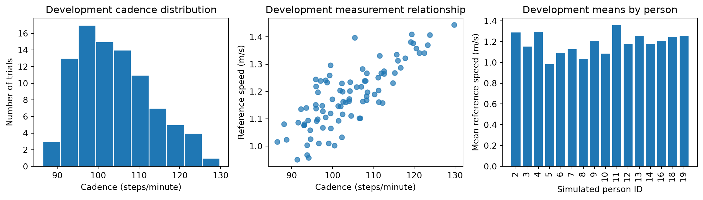
A histogram asks where individual values concentrate and whether the distribution has gaps, skew, or multiple peaks. Its appearance depends on bin boundaries; an apparent pattern that vanishes after a small bin change deserves caution. A scatterplot asks how two measured variables vary together. A per-person summary asks whether pooled behavior hides group differences. No one plot answers all three.
The NIST introduction to exploratory data analysis describes exploration as an approach to learning about structure and checking assumptions, with graphics playing a central role. Use that attitude here: a plot creates questions to investigate, not automatic evidence of a mechanism.
11.6.1 Step 4: Plot development data with units
# Step 4: Compare distributions, relationships, and participant summaries.# Use complete measurement pairs only for the two-variable scatterplot.complete_development_pairs = development_measurements.dropna()# Average trial speeds within each person to expose the grouping structure.mean_speed_per_person = development_trials.groupby("person_id")["reference_speed_meters_per_second"].mean()# Allocate three panels for three distinct exploratory questions.figure, axes = plt.subplots(1, 3, figsize=(12, 3.5))# Show the range and frequency of available cadence measurements.axes[0].hist( development_measurements["cadence_steps_per_minute"].dropna(), bins=10, edgecolor="white")axes[0].set_title("Development cadence distribution")axes[0].set_xlabel("Cadence (steps/minute)")axes[0].set_ylabel("Number of trials")# Compare paired cadence and reference-speed measurements.axes[1].scatter( complete_development_pairs["cadence_steps_per_minute"], complete_development_pairs["reference_speed_meters_per_second"], alpha=0.7)axes[1].set_title("Development measurement relationship")axes[1].set_xlabel("Cadence (steps/minute)")axes[1].set_ylabel("Reference speed (m/s)")# Display one mean per person rather than treating each trial as independent.axes[2].bar(mean_speed_per_person.index.astype(str), mean_speed_per_person)axes[2].set_title("Development means by person")axes[2].set_xlabel("Simulated person ID")axes[2].set_ylabel("Mean reference speed (m/s)")axes[2].tick_params(axis="x", labelrotation=90)figure.tight_layout()plt.show()
Figure 11.1: Development data only: cadence distribution, paired measurements, and mean speed within each simulated person. Repeated trials do not supply additional independent people.
Read the scatter as a relationship within this constructed development set. Its spread is expected because simulated people differ in unobserved step length and the target includes noise. The per-person bars make the grouping visible but do not provide uncertainty intervals. Sorting IDs or colors cannot turn these means into an estimate for a real population.
Pearson correlation summarizes a linear association between two nonconstant measurements:
Here \(x_i\) is cadence, \(y_i\) is speed, and \(m\) counts their complete pairs. The units cancel, so \(r\) is dimensionless. It lies between \(-1\) and \(1\) for nonzero denominators. A value near zero does not exclude a curved association; a strong value does not prove that changing one variable would cause the other to change. The pooling of different people can also create an association different from within-person behavior.
# Step 5: Quantify the pooled linear relationship using complete pairs.# Store pairwise correlations; the diagonal contains self-correlations.correlation_table = complete_development_pairs.corr(method="pearson")# Read the off-diagonal entry connecting cadence with reference speed.cadence_speed_correlation = correlation_table.loc["cadence_steps_per_minute", "reference_speed_meters_per_second"]print("Complete pairs:", len(complete_development_pairs))print("Pooled Pearson correlation:", round(cadence_speed_correlation, 3))assert np.isfinite(cadence_speed_correlation)
Complete pairs: 90
Pooled Pearson correlation: 0.801
In the checked run, the development set contains 90 complete cadence-speed pairs, with pooled correlation 0.801. Six of its 96 cadence readings are missing, a fraction of 0.0625. These values are outputs of the specified simulation and split. The strong association reflects how the artificial target was constructed; it is not a measured result about human walking.
Dropping rows here defines which pairs enter a descriptive calculation. It is not a recommendation to delete missing rows before model evaluation. If missingness is systematic, complete cases can represent a different population. The preparation chapter uses an imputer fitted on training data instead.
11.7 Convert findings into a defensible plan
An exploration should end with decisions and unanswered questions. For this example, retain participant and trial IDs for traceability, exclude them from predictors, keep the participant holdout, and plan training-only imputation for missing cadence. Compare a sensor-based predictor with a training-set constant baseline using an error metric in m/s. Evaluate on held-out people only after the development procedure is fixed. These decisions follow the stated task and constructed table, not a measured claim of predictive usefulness.
For a real study, add questions the synthetic data cannot answer. Are the portable-sensor and reference measurements synchronized? How accurate is the reference system? Are trials drawn from the intended range of speeds and environments? Are there enough independently sampled people? Could device identity or site encode the label? The answers may require revisiting collection before model choice.
Outliers deserve investigation rather than automatic deletion. An extreme value may be a unit error, a sensor fault, a genuine rare event, or an important part of the intended population. Predetermine physical validity rules when possible; learn statistical thresholds within training data. If a rule excludes difficult but legitimate cases, report the narrowed target population.
A duplicate row can also mean different things. Two identical exported records may be an accidental duplication; two distinct trials can coincidentally have identical rounded measurements. Check the record key and provenance before deleting either. Overlapping windows from the same recording require a split that prevents shared information crossing the boundary, even when their feature rows are not identical.
11.8 Exercises and worked answers
Observation versus sampling unit. A table has 12,000 windows from 24 people. Is its sample size 12,000 or 24?
Answer: It has 12,000 rows and 24 participant sampling units. The appropriate amount of independent information depends on the question and dependence structure. For evaluating predictions on new people, splitting by participant and reporting participant counts are essential; the row count alone is inadequate.
Unavailable feature. A predictor uses a therapist’s assessment written after reviewing the complete session to make a prediction at the first minute. What is wrong?
Answer: The assessment may contain later-session information unavailable at prediction time. It can potentially serve as part of label construction, if justified, but cannot be an input for that timing requirement. Redefine the inputs or explicitly change the prediction time.
Calculate a summary. Available readings are 90, 100, and 110 steps/minute, with one additional missing reading. Find the mean, sample standard deviation, and missing fraction.
Answer: The mean is 100. The squared deviations sum to 200; dividing by \(3-1\) and taking a square root gives 10 steps/minute. The missing fraction is \(1/4=0.25\). Dividing the sum by four would incorrectly treat the missing reading as zero.
Interpret correlation. A strong pooled relationship between cadence and speed is found. Does that establish a personal response to a cadence intervention?
Answer: No. Between-person differences, other variables, and the measurement process may contribute. A pooled predictive association is not an intervention effect. The synthetic construction also provides no real-world evidence for an intervention.
Practical extension. Change trials_per_person to 12, regenerate the table, and rerun the exploration. What has increased?
Answer: The row count and repeated measurements increase; the number of simulated people remains 20. The final-test group still contains four people. More within-person observations may improve estimates for those people but do not supply additional independent participant coverage.
Label claim. A dataset marks treadmill walking as class 0 and a deliberately altered walking condition as class 1. Can a resulting classifier be described as detecting pathology?
Answer: Those labels establish the recorded condition contrast. A pathology claim requires suitable clinical label definitions and evidence for the intended population and use. Reword the task around what the labels actually measure.
11.9 Revision summary
Write the task before the model: observation, target, units, prediction time, available inputs, intended population, metric, and baseline. Distinguish row counts from independent sampling units. Preserve provenance and audit labels separately from features. Reserve a task-appropriate test set before detailed exploration. Use numerical summaries and complementary plots on development data, retaining units and missingness. Investigate unusual records using their provenance. Convert patterns into explicit, testable development choices, and keep predictive association separate from causal or clinical claims.
The next chapter, Chapter 12, turns this plan into a reproducible experiment. Chapter 13 then shows how preparation can remain inside every training fold.