7  Probability and uncertainty

7.1 Why a prediction needs uncertainty

Two observations can have similar measured features and different targets. Sensors have noise, unmeasured factors vary, and a training sample covers only part of the population we care about. Probability gives a language for these uncertainties. It helps distinguish a model saying “class 1 is more plausible” from a model claiming certainty, and it explains why repeated experiments can produce different numerical results.

We first define events and random variables, then distributions, expectation, variance, conditional probability, and Bayes’ rule. A final section introduces entropy, which later helps explain decision-tree splitting. All numerical settings in this chapter are invented teaching models rather than estimates from a real sensor study.

Prerequisites: arithmetic, sums, logarithms, and functions from Chapter 5. The executable examples use NumPy and Matplotlib. No integration techniques are needed; an integral is introduced as area under a density.

Learning objectives:

1. Distinguish an outcome, an event, and a random variable.
2. Read discrete probabilities and continuous densities correctly.
3. Calculate expectation and variance in a small finite model.
4. Use conditional probability, independence, and Bayes’ rule with explicit assumptions.
5. Interpret simulated frequencies and entropy without overclaiming certainty.

7.2 Outcomes, events, and probability

An outcome is one possible result of an experiment. The sample space \(\Omega\) is the set of possible outcomes. An event is a subset of that space. For two binary sensor checks, the outcomes might be \(\Omega=\{00,01,10,11\}\). The event “exactly one check is positive” contains \(01\) and \(10\). The label 1 means positive in this example; it is a definition, not a claim that positive is desirable.

A probability assignment \(P\) obeys three rules: \(P(A)\geq0\) for every event \(A\), \(P(\Omega)=1\), and probabilities of disjoint events add. Disjoint events cannot happen together. These rules imply \(P(A^c)=1-P(A)\), where \(A^c\) is the event that \(A\) does not happen, and

\[ P(A\cup B)=P(A)+P(B)-P(A\cap B). \]

Here \(\cup\) means “or, including both,” and \(\cap\) means “and.” Subtracting the intersection corrects the double counting of outcomes in both events. Probabilities are dimensionless and lie between zero and one.

Equal probability for every outcome is a modeling assumption, not a rule. Counting favorable outcomes and dividing by the total works only when the outcomes being counted are equally likely. Similarly, observing no occurrences in a small sample does not establish a true event probability of zero.

7.3 Random variables and distributions

A random variable maps outcomes to numbers. Capital \(X\) names the uncertain quantity; lowercase \(x\) denotes a possible or observed value. For example, \(X\) can count positive sensor checks. A distribution describes how probability is allocated across possible values of the random variable. Randomness describes our model before the value is observed; an observed number is not still changing merely because its generating process was random.

A discrete variable has a finite or countably infinite set of possible values. Its probability mass function, \(p_X(x)=P(X=x)\), is nonnegative and satisfies \(\sum_x p_X(x)=1\). A continuous variable such as an idealized time measurement has a density \(f_X(x)\) satisfying

\[ f_X(x)\geq0,\qquad \int_{-\infty}^{\infty}f_X(x)\,dx=1, \qquad P(a\leq X\leq b)=\int_a^b f_X(x)\,dx. \]

An integral here represents accumulated area. A density value is not the probability at one point. For a variable with a continuous density, \(P(X=x)=0\) for any individual \(x\), while intervals can have positive probability. Density can exceed one: a uniform variable on an interval of length 0.1 has density 10 there, and total area is still one. A density has inverse measurement units, so density times an interval width is dimensionless.

The cumulative distribution function is \(F_X(t)=P(X\leq t)\) for either type of variable. It is nondecreasing, lies between zero and one, and tends toward zero and one at the respective extremes. Cumulative probability and density answer different questions.

7.4 Useful distribution families

7.4.1 Bernoulli and binomial variables

A Bernoulli variable takes value 1 with probability \(p\) and 0 with probability \(1-p\), where \(0\leq p\leq1\). It is a model for one binary outcome. Its mass function can be written \(P(X=x)=p^x(1-p)^{1-x}\) for \(x\in\{0,1\}\), with endpoint cases understood directly rather than by ambiguous expressions such as \(0^0\).

If \(K\) counts successes in \(m\) independent Bernoulli trials with the same success probability \(p\), it has a binomial distribution:

\[ P(K=k)=\binom{m}{k}p^k(1-p)^{m-k},\quad k=0,\ldots,m. \]

The binomial coefficient \(\binom{m}{k}=m!/[k!(m-k)!]\) counts the sequences containing \(k\) successes. Factorial means multiplying positive integers up to the given number, with \(0!=1\). With \(m=3\), \(p=0.5\), exactly two successes have probability \(3(0.5)^2(0.5)=3/8\). Dependent trials or a changing success probability do not satisfy this model.

7.4.2 Uniform and normal variables

A continuous uniform distribution on \([a,b]\), \(a<b\), has constant density \(1/(b-a)\) within the interval and zero outside. Equal-length subintervals have equal probability. This is a statement about intervals, not positive point probabilities.

A normal, or Gaussian, variable has mean parameter \(\mu\) and positive standard deviation parameter \(\sigma\):

\[ f_X(x)=\frac{1}{\sigma\sqrt{2\pi}} \exp\left[-\frac{(x-\mu)^2}{2\sigma^2}\right]. \]

We write \(X\sim\mathcal N(\mu,\sigma^2)\); the second argument here is the variance. The symbol \(\sim\) means “is distributed as.” The center is \(\mu\), the scale is \(\sigma\), and the exponent is dimensionless. A normal model allows every real value, so it can be inappropriate for nonnegative quantities near a hard boundary. A bell-shaped histogram alone does not verify independence or establish a physical noise mechanism.

7.4.3 Poisson counts

For a nonnegative count \(K\), a Poisson model uses a parameter \(\lambda>0\): \(P(K=k)=e^{-\lambda}\lambda^k/k!\) for \(k=0,1,\ldots\). Its mean and variance both equal \(\lambda\). It is useful for some event counts over a specified exposure, provided the model’s rate and dependence assumptions are appropriate. A count of events per hour and a count per minute require different rate parameters. Not every count dataset has equal mean and variance; the Poisson form is a candidate model, not a mandatory default.

7.5 Expectation is a probability-weighted average

For a finite discrete variable,

\[ \mathbb E[X]=\sum_x x p_X(x)=\mu. \]

The notation \(\mathbb E\) means expectation under the specified distribution. If \(X\) takes values 0, 1, and 2 with probabilities 0.2, 0.5, and 0.3, then \(\mu=0(0.2)+1(0.5)+2(0.3)=1.1\). The expected value need not be one of the possible outcomes. It describes the distribution’s average, not the outcome guaranteed on the next trial.

For a function \(g\), \(\mathbb E[g(X)]=\sum_x g(x)p_X(x)\) when the sum exists. Expectation is linear: \(\mathbb E[aX+bY]=a\mathbb E[X]+b\mathbb E[Y]\) for constants \(a,b\) and random variables with finite expectations. Independence is not needed for that identity. However, \(\mathbb E[X^2]\) generally differs from \((\mathbb E[X])^2\). For a fair binary variable the former is 0.5 and the latter is 0.25.

The variance measures expected squared deviation from the mean:

\[ \operatorname{Var}(X)=\mathbb E[(X-\mu)^2] =\mathbb E[X^2]-\mu^2=\sigma^2. \]

To obtain the last equality, expand the square: \(\mathbb E[X^2-2\mu X+\mu^2] =\mathbb E[X^2]-2\mu\mathbb E[X]+\mu^2\). Then substitute \(\mathbb E[X]=\mu\). The standard deviation \(\sigma\) is the nonnegative square root of variance, restoring the original units. For the three-value example, \(\mathbb E[X^2]=1.7\) and variance is \(1.7-1.21=0.49\).

For a Bernoulli variable, \(X^2=X\), so its variance is \(p-p^2=p(1-p)\). For independent finite-variance variables, variances add. Thus a binomial count has mean \(mp\) and variance \(mp(1-p)\). Without independence, covariance terms must be included, as developed in Chapter 8. For a constant \(a\), variance obeys \(\operatorname{Var}(aX+b)=a^2\operatorname{Var}(X)\).

The probability-weighted interpretation is discussed in OpenStax’s section on expected value and standard deviation. The calculations here use our own finite teaching model.

7.5.1 Verify a complete discrete model

1. Check that all masses are nonnegative and sum to one.
2. Multiply each outcome by its mass and sum.
3. Accumulate squared deviations using the same masses.
4. Compare with the second-moment identity.

# Step 1: Import tools and store a complete finite probability model.
import numpy as np

# Possible counts for one artificial experiment.
possible_counts = np.array([0.0, 1.0, 2.0])
# Probability mass for each count, in matching order.
probability_masses = np.array([0.2, 0.5, 0.3])
assert np.all(probability_masses >= 0.0)
assert np.isclose(np.sum(probability_masses), 1.0)

# Step 2: Expand the probability-weighted mean term by term.
# Start the weighted total at zero before accumulating contributions.
expected_count = 0.0
for outcome_index in range(len(possible_counts)):
    # Each outcome contributes in proportion to its probability mass.
    weighted_outcome = (
        possible_counts[outcome_index] * probability_masses[outcome_index]
    )
    expected_count = expected_count + weighted_outcome

# Step 3: Calculate spread under the distribution, rather than over equally weighted values.
# Deviation is measured from the model's expected count.
count_deviations = possible_counts - expected_count
# Weight squared deviations by their actual probability masses.
count_variance = np.sum(probability_masses * count_deviations ** 2)
# The second moment provides a separate algebraic check.
second_moment = np.sum(probability_masses * possible_counts ** 2)
assert np.isclose(expected_count, 1.1)
assert np.isclose(count_variance, 0.49)
assert np.isclose(count_variance, second_moment - expected_count ** 2)
print("Expected count:", expected_count)
print("Count variance:", count_variance)

Expected count: 1.1
Count variance: 0.49

Using np.mean(possible_counts) would give 1 rather than 1.1 because it would implicitly assign equal weights. Likewise, np.var(possible_counts) would describe a different equally weighted empirical distribution. Correct code must represent the intended probability model, not merely use a function with a plausible name.

7.6 Conditional probability and independence

Conditional probability restricts attention to cases in which another event occurred. If \(P(B)>0\),

\[ P(A\mid B)=\frac{P(A\cap B)}{P(B)}, \qquad P(A\cap B)=P(A\mid B)P(B). \]

The vertical bar means “given.” For 100 artificial inspections, suppose 20 have a warning and 8 have both a warning and a confirmed defect. Among warning cases, the defect fraction is \(8/20=0.4\). The denominator is the conditioning group, not all 100 inspections.

Events \(A,B\) are independent when \(P(A\cap B)=P(A)P(B)\). If \(P(B)>0\), this implies \(P(A\mid B)=P(A)\). Independence means that learning whether \(B\) occurred does not change the event probability of \(A\). Disjoint positive-probability events are not independent: knowing one happened rules the other out. Statistical independence is stronger than zero linear correlation.

For a sequence of random variables, independent and identically distributed (IID) means their joint distribution factors into individual distributions and each follows the same distribution. Repeated windows from one person’s sensor recording are often dependent; numbering them as separate rows does not make them IID. Independence assumptions affect uncertainty estimates and evaluation protocols, not just mathematical notation.

7.7 Bayes’ rule and base rates

The product rule can be written in two directions: \(P(A\cap B)=P(B\mid A)P(A)=P(A\mid B)P(B)\). Dividing by \(P(B)>0\) gives Bayes’ rule:

\[ P(A\mid B)=\frac{P(B\mid A)P(A)}{P(B)}. \]

For an event \(A\) with \(0<P(A)<1\), total probability gives

\[ P(B)=P(B\mid A)P(A)+P(B\mid A^c)P(A^c). \]

Suppose a manufactured part has a defect with probability 0.02. An inspection flags 90% of defective parts and 10% of nondefective parts. Define \(D\) as “defective” and \(F\) as “flagged.” Then \(P(F)=0.9(0.02)+0.1(0.98)=0.116\), so \(P(D\mid F)=0.018/0.116\approx0.1552\). The fraction is much smaller than 0.9 because nondefective parts are far more common.

This is a hypothetical quality-control calculation. Its conclusion depends on all three assumed probabilities and the population to which they apply. Changing the defect base rate changes the posterior even when the conditional inspection rates remain fixed. A classifier’s score also need not be a well-calibrated probability merely because it lies between zero and one.

# Step 4: Define the hypothetical population and inspection mechanism.
# The base rate describes defects before observing the inspection flag.
defect_probability = 0.02
# The flag rate among genuinely defective parts.
flag_given_defect = 0.90
# The flag rate among parts without a defect.
flag_given_no_defect = 0.10

# Step 5: Combine the two mutually exclusive ways to obtain a flag.
# This joint probability represents parts that are defective and flagged.
defect_and_flag = defect_probability * flag_given_defect
# This joint probability represents nondefective parts that are flagged.
no_defect_and_flag = (1.0 - defect_probability) * flag_given_no_defect
# Total probability supplies the denominator required by Bayes' rule.
flag_probability = defect_and_flag + no_defect_and_flag
# Restrict the defective-and-flagged group to the complete flagged population.
defect_given_flag = defect_and_flag / flag_probability
print("Probability of a flag:", flag_probability)
print("Probability of a defect given a flag:", defect_given_flag)
assert np.isclose(flag_probability, 0.116)
assert 0.15 < defect_given_flag < 0.16

Probability of a flag: 0.116
Probability of a defect given a flag: 0.15517241379310345

7.8 Simulation and the law of large numbers

Simulation generates artificial observations from a specified model. It can illustrate a theorem’s implications, check arithmetic, or investigate an estimator. It cannot establish that the generating assumptions describe a real dataset. Under IID sampling with a finite mean, a sample average approaches the population mean in the law-of-large-numbers sense as sample size grows. This does not promise that every additional observation improves the current estimate or that a particular finite sample will be close.

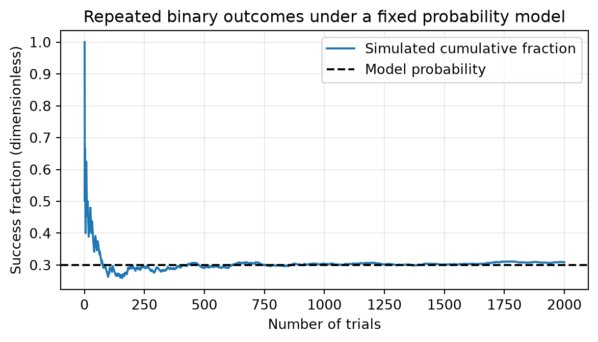
We simulate Bernoulli trials with probability 0.3 and inspect cumulative fractions. A fixed seed makes this run repeatable in the same software setup; it does not remove sampling variability from the underlying experiment. NumPy documents the meanings of n and p in its Generator.binomial API. Here n=1 creates individual binary trials.

# Step 6: Generate repeatable independent binary outcomes from the teaching model.
import matplotlib.pyplot as plt

# Fix the seed so readers can compare the same artificial sequence.
random_seed = 42
# The generator owns the random state used in this chapter.
random_generator = np.random.default_rng(random_seed)
# This is the model's true success probability, known because we set it.
success_probability = 0.30
# Keep the sample small enough for an ordinary laptop.
number_of_trials = 2000
# n=1 means one Bernoulli outcome per returned entry.
binary_outcomes = random_generator.binomial(
    n=1, p=success_probability, size=number_of_trials
)

# Step 7: Calculate the fraction observed after each successive trial.
# The first denominator is one; division by zero is therefore avoided.
trial_counts = np.arange(1, number_of_trials + 1)
# np.cumsum stores the number of successes encountered up to each position.
cumulative_successes = np.cumsum(binary_outcomes)
# Divide each cumulative count by the matching number of completed trials.
cumulative_fractions = cumulative_successes / trial_counts
print("Final simulated success fraction:", cumulative_fractions[-1])

# Step 8: Compare the fluctuating observed fraction with the known model probability.
figure, axis = plt.subplots(figsize=(6.2, 3.6))
axis.plot(trial_counts, cumulative_fractions, label="Simulated cumulative fraction")
axis.axhline(success_probability, color="black", linestyle="--", label="Model probability")
axis.set_xlabel("Number of trials")
axis.set_ylabel("Success fraction (dimensionless)")
axis.set_title("Repeated binary outcomes under a fixed probability model")
axis.legend()
axis.grid(alpha=0.25)
figure.tight_layout()
plt.show()

Final simulated success fraction: 0.309

Figure 7.1: Simulated cumulative success fractions under a fixed Bernoulli model. Local fluctuations do not contradict a long-run probability model.

The curve may cross the reference line or move farther away over some intervals. Those fluctuations are compatible with convergence in the long run. Choosing only a favorable seed would hide this variability. Repeating with several preselected seeds is an optional sensitivity exercise, not a way to select a preferred scientific conclusion.

7.9 Entropy: uncertainty over categorical outcomes

For class probabilities \(p_1,\ldots,p_K\), Shannon entropy in bits is

\[ H=-\sum_{k=1}^{K}p_k\log_2 p_k. \]

We define a zero-probability contribution as zero, consistent with the limit \(p\log p\to0\) as \(p\to0^+\). A binary distribution with probabilities \((1,0)\) has entropy zero, whereas \((0.5,0.5)\) has entropy one bit. For a fixed \(K\), the uniform distribution has maximum entropy \(\log_2 K\). Changing to natural logarithms changes the unit to nats, not the ordering.

Entropy measures uncertainty in a categorical distribution. It is not classification accuracy, and a high-entropy node does not prove that useful feature splits exist. Later, a tree will compare the parent’s entropy with a weighted average of child entropies. Weighting matters because a tiny pure child should not receive the same influence as a large mixed child.

# Step 9: Calculate entropy while handling zero masses deliberately.
# These artificial class fractions form a certain and an uncertain distribution.
class_distributions = [np.array([1.0, 0.0]), np.array([0.5, 0.5])]
for class_probabilities in class_distributions:
    # Select positive entries before applying log2, since log2(0) is undefined.
    positive_probabilities = class_probabilities[class_probabilities > 0.0]
    # The omitted zero entries contribute zero by the limiting convention.
    entropy_bits = -np.sum(positive_probabilities * np.log2(positive_probabilities))
    print("Class probabilities:", class_probabilities, "Entropy (bits):", entropy_bits)

Class probabilities: [1. 0.] Entropy (bits): -0.0
Class probabilities: [0.5 0.5] Entropy (bits): 1.0

7.10 Exercises and worked answers

1. Use the union rule. If \(P(A)=0.4\), \(P(B)=0.3\), and \(P(A\cap B)=0.1\), find \(P(A\cup B)\).
   Answer: \(0.4+0.3-0.1=0.6\). The overlap was counted twice before subtraction.
2. Distinguish density and probability. A uniform variable on \([0,0.2]\) has what density and what probability of lying in \([0,0.1]\)?
   Answer: density 5 and interval probability \(5(0.1)=0.5\). The probability at exactly 0.1 is zero under this continuous model.
3. Calculate a binary variance. For success probability 0.2, find mean and variance of one Bernoulli outcome.
   Answer: mean 0.2 and variance \(0.2(0.8)=0.16\).
4. Check independence. Two positive-probability events are disjoint. Can they be independent?
   Answer: no. Their intersection probability is zero, while the product of their separate positive probabilities is positive.
5. Apply the binomial model. What is the probability of zero successes in four independent trials with success probability 0.1?
   Answer: \((0.9)^4=0.6561\). Independence and common success probability justify multiplication of the four failure probabilities.
6. Interpret entropy. Compare \((0.5,0.5)\) with \((0.9,0.1)\).
   Answer: the first has one bit; the second has \(-0.9\log_2 0.9-0.1\log_2 0.1\approx0.469\) bits. The second is more concentrated, but this does not tell us whether a predictor is correct.
7. Explain a sample fluctuation. A probability-0.3 process produces 38 successes in 100 trials. Does it refute the probability model?
   Answer: not by itself. Finite samples fluctuate. A formal model check would quantify how unusual the result is under the assumptions and consider the sampling process, rather than require exact equality to 30.

7.11 One-page revision summary

Quantity	Interpretation and condition
\(P(A\mid B)\)	Probability within event \(B\); requires \(P(B)>0\).
Independence	Joint probability factors; distinct from disjointness.
Mass versus density	Mass gives point probabilities; density gives interval area.
\(\mathbb E[X]\)	Probability-weighted average, not a guaranteed next outcome.
\(\operatorname{Var}(X)\)	Expected squared deviation; standard deviation restores units.
Bernoulli / binomial	One binary trial / count from independent identical trials.
Normal	Real-valued location/scale model; variance is \(\sigma^2\).
Bayes’ rule	Updates an event probability using evidence and the base rate.
Entropy	Categorical uncertainty; specify the logarithm base.

Probability starts with a proposed data-generating model and works toward possible observations. Chapter 8 reverses that perspective: given a finite sample, what can we estimate about the unknown population, and how uncertain should the estimate be?