A useful first prediction model should be simple enough to inspect. Linear regression gives us a complete example of learning: choose a family of predictions, measure error, estimate parameters, and check performance on observations that were not used to fit the parameters. Its simplicity also makes wrong assumptions easier to see.
After this chapter you should be able to:
Derive the squared-error objective and its gradient, including the intercept.
Fit a line by hand and fit several features using explicit gradient descent.
Explain the normal equations and why an explicit matrix inverse is usually a poor numerical implementation.
Compare an educational implementation with scikit-learn on the same data.
Recognize curvature, outliers, unstable coefficients, extrapolation, and leakage.
Evaluate continuous predictions using a baseline, MAE, RMSE, and \(R^2\).
Read Chapter 6, Chapter 9, Chapter 10, Chapter 12, and Chapter 13 first. Probability and estimation are needed for the statistical interpretation, rather than merely computing a least-squares fit. Run this chapter’s code cells in order from a fresh session; no variables from another chapter are required.
14.2 Problem definition and motivation
Suppose we have a small sensor calibration table. Each row records an applied force, the ambient temperature, and a sensor response. We want to predict the response for a new force and temperature within the calibration range. A simple model is
\[
\hat y_i=b+w_1x_{i1}+w_2x_{i2}.
\]
Here \(i\) indexes observations, \(x_{i1}\) is force in newtons (N), \(x_{i2}\) is temperature in degrees Celsius, and \(\hat y_i\) is predicted response in volts (V). The intercept \(b\) has units V. The coefficients \(w_1\) and \(w_2\) have units V/N and V/degree Celsius respectively. Changing the temperature scale changes the intercept; coefficients are meaningful only together with feature definitions and units.
This is regression because the target is continuous. Predicting a walking condition or a species is a classification problem and requires different assumptions and evaluation. A calibration relationship is also not automatically a causal effect: the way the data were collected matters.
Our experiment uses deliberately synthetic independent observations. It is an arithmetic teaching model, not a measured calibration study. The later exercise about grouped recordings explains why a random row split would be inappropriate for some sensor applications.
14.3 Intuition
With one feature, each parameter choice draws a line. The intercept moves the line up or down, and the slope rotates it. The residual is observed minus predicted target:
\[e_i=y_i-\hat y_i.\]
Positive residuals mean underprediction. We square residuals so positive and negative errors cannot cancel, and so large errors have greater influence. Squaring is a modeling choice: it makes a badly corrupted observation especially influential.
Consider three observations, with feature values \(0,1,2\) and target values \(1,2,2\). Their means are \(\bar x=1\) and \(\bar y=5/3\). For a line with a freely fitted intercept, the least-squares slope is
Predictions are \(7/6,10/6,13/6\), and residuals are \(-1/6,1/3,-1/6\). Their sum is zero. The sum of squared residuals is \(1/6\), so MSE is \(1/18\). A line need not pass through any observation to minimize total squared error. It does pass through \((\bar x,\bar y)\) when an intercept is fitted by ordinary unweighted least squares.
14.4 Mathematical foundations
14.4.1 Model, dimensions, and loss
Let \(n\) be the number of training observations and \(p\) the number of features. Store features in \(X\in\mathbb R^{n\times p}\) and targets in \(\mathbf y\in\mathbb R^n\). Row \(\mathbf x_i^T\) contains one observation. Collect slopes in \(\mathbf w\in\mathbb R^p\) and use a separate intercept \(b\in\mathbb R\). The predicted vector is
\[\hat{\mathbf y}=X\mathbf w+b\mathbf 1.\]
Add a leading column of ones to form the design matrix\(A=[\mathbf1\ X]\in\mathbb R^{n\times(p+1)}\), and let \(\boldsymbol\theta=(b,w_1,\ldots,w_p)^T\). Then \(\hat{\mathbf y}=A\boldsymbol\theta\). This absorbs the intercept into the matrix notation without changing the model. The foundations chapters used \(D\) and \(\boldsymbol\beta\) for the same design-matrix and parameter roles; here they are renamed \(A\) and \(\boldsymbol\theta\), without changing the construction.
The factor \(1/2\) simplifies derivatives. It does not change the minimizer. MSE is \(2J\), rather than \(J\); forgetting this factor changes the gradient and effective learning rate. Both \(J\) and MSE have squared target units.
14.4.2 Deriving the gradient
Let \(r_i=\hat y_i-y_i=-e_i\) be prediction error, so the code’s error sign matches the derivative. By the chain rule,
Each feature contributes to the gradient in proportion to both its value and the current error. A positive gradient means a small increase in that parameter raises loss, so gradient descent subtracts it. In augmented notation,
\(A^T\) has shape \((p+1)\times n\), so the gradient has \(p+1\) entries, matching the parameter vector. The learning rate \(\eta>0\) controls the update size; scaling features affects which values are numerically useful.
14.4.3 Normal equations and numerical solving
At an unconstrained minimum, the gradient vanishes:
\[A^TA\hat{\boldsymbol\theta}=A^T\mathbf y.\]
If the columns of \(A\) are linearly independent, \(A^TA\) is invertible and the unique solution can be written
This formula is a derivation, not a recommendation to calculate an inverse. Forming \(A^TA\) squares the 2-norm condition number for a full-column-rank matrix, worsening sensitivity to roundoff when columns are nearly dependent. QR or singular-value-based least-squares solvers avoid forming the inverse. With dependent columns, coefficients need not be unique, even though fitted training predictions are the unique projection onto the column space of \(A\). A least-squares solver can choose a minimum-norm coefficient vector. See NumPy’s least-squares solver documentation.
The Hessian is \(A^TA/n\), which is positive semidefinite since for every vector \(\mathbf v\), \(\mathbf v^TA^TA\mathbf v=\|A\mathbf v\|^2\geq0\). The objective is therefore convex: every stationary point is a global minimum. Positive definiteness, and hence a unique coefficient solution, requires full column rank. For full-batch descent on this quadratic, \(0<\eta<2/\lambda_{\max}(A^TA/n)\) ensures contraction in directions with positive eigenvalues; standardizing features helps but does not guarantee that any chosen rate will converge.
14.4.4 What least squares estimates
If \(Y=\mathbf a^T\boldsymbol\theta+\varepsilon\), with \(E[\varepsilon\mid\mathbf a]=0\) and finite second moments, the linear conditional mean is correctly specified. For a generic predictor \(g(\mathbf x)\),
To obtain this identity, write \(Y-g=(Y-E[Y\mid\mathbf x])+(E[Y\mid\mathbf x]-g)\), expand the square, and use the zero conditional mean of the first term to eliminate the cross term. Squared loss targets the conditional mean. If it is nonlinear, least squares still finds the best training fit in the selected linear feature space; this does not make that space correct.
Gaussian noise is not needed to compute least squares. If, conditional on the design matrix \(A\), the error vector follows \(\boldsymbol\varepsilon\mid A\sim\mathcal N(\mathbf0,\sigma^2I)\), the negative log-likelihood, for fixed \(\sigma\), differs from the sum of squares only by a positive multiplier and a parameter-independent constant. Here \(I\) is the \(n\times n\) identity matrix. That stronger model makes least squares a maximum-likelihood estimator and supports classical normal-theory inference under its conditions.
14.5 How the algorithm works
The from-scratch version uses full-batch gradient descent:
Reserve test observations. Split the remaining development observations into training and validation sets.
Compute feature means and standard deviations using training data only.
Standardize all partitions using those same training statistics. Prepend a column of ones.
Initialize one parameter per design-matrix column to zero.
Predict all training targets, calculate errors, and average each column’s error-weighted contribution.
Subtract the learning rate times the gradient. Repeat until the gradient is small or the iteration limit is reached.
Check convergence, compare validation performance, and evaluate the fixed model on the final test set.
Pseudocode, with \(d=p+1\):
theta = d zeros
repeat up to maximum_iterations:
    prediction = A times theta
    error = prediction - target
    for column j:
        gradient[j] = mean(error * A[:, j])
    if norm(gradient) <= tolerance: stop
    theta = theta - learning_rate * gradient
return theta and loss history
The intercept is a column of ones, so its update uses the mean error. Do not standardize that column: its standard deviation is zero.
14.6 From-scratch implementation
14.6.1 Step 1: Generate and partition a synthetic calibration problem
We deliberately use a known linear generating relationship to check implementation correctness. There are 180 rows, two features, and independent zero-mean noise with standard deviation 0.08 V. Knowing the generator is a privilege of synthetic data, not something available in most projects. A fixed seed recreates the draws for this environment; it does not prove performance is insensitive to data sampling.
# Step 1: Import numerical, table, plot, and splitting tools.import numpy as npimport pandas as pdimport matplotlib.pyplot as pltfrom sklearn.model_selection import train_test_split# Configure the synthetic experiment and preserve repeatable random draws.# Number of independent synthetic calibration measurements.number_of_observations =180# Seed controls the generated measurements and partitioning.random_seed =42# Local generator avoids changing NumPy's global random state.random_generator = np.random.default_rng(random_seed)# Generate the two measured input quantities in their original units.# Applied force, in newtons, spans the calibration range.force_newtons = random_generator.uniform(0.0, 30.0, number_of_observations)# Ambient temperature, in degrees Celsius, is independently varied.temperature_celsius = random_generator.uniform(15.0, 35.0, number_of_observations)# Measurement noise, in volts, prevents a perfectly deterministic fit.noise_volts = random_generator.normal(0.0, 0.08, number_of_observations)# Response follows an invented linear calibration rule, in volts.response_volts = (0.4+0.06* force_newtons+0.015* (temperature_celsius -20.0) + noise_volts)# Feature matrix has one observation per row and two columns.features = np.column_stack((force_newtons, temperature_celsius))# Reserve the final test set before any model or preprocessing is fitted.# The four outputs keep each feature row aligned with its response.development_features, testing_features, development_targets, testing_targets = train_test_split( features, response_volts, test_size=0.20, random_state=random_seed)# A quarter of the remaining 80% gives a 20% validation set overall.training_features, validation_features, training_targets, validation_targets = train_test_split( development_features, development_targets, test_size=0.25, random_state=random_seed)print("Training/validation/test shapes:", training_features.shape, validation_features.shape, testing_features.shape)assert training_features.shape == (108, 2)assert validation_features.shape == (36, 2)assert testing_features.shape == (36, 2)
This split estimates performance on independent new draws from the same generator. A real repeated-participant calibration study may require participant or device groups to be kept together. Chronological deployment may instead require a time-based split; see Chapter 12.
14.6.2 Step 2: Fit preprocessing using training rows
Standardization replaces feature \(j\) by \(z_{ij}=(x_{ij}-\mu_j)/s_j\). Here \(\mu_j\) and \(s_j\) are the training mean and population-form standard deviation (divisor \(n\)), used as numerical scaling statistics. This is not an unbiased estimate of population variance. An intercept makes the unregularized prediction family unchanged by an invertible affine feature transformation.
# Step 2: Learn scaling statistics exclusively from training features.# One mean per feature, with shape (2,).training_means = training_features.mean(axis=0)# One positive standard deviation per feature, also shape (2,).training_scales = training_features.std(axis=0, ddof=0)assert np.all(training_scales >0.0)# Apply the same learned transformation to every partition.# Scaled training rows are used to estimate regression coefficients.scaled_training_features = (training_features - training_means) / training_scales# Validation rows must not determine their own scaling statistics.scaled_validation_features = (validation_features - training_means) / training_scales# Test features are transformed without using their targets or refitting.scaled_testing_features = (testing_features - training_means) / training_scales# Create design matrices; a leading one implements the intercept.# Shape is (108, 3): one intercept column and two scaled features.training_design = np.column_stack((np.ones(len(training_targets)), scaled_training_features))# Validation and test matrices have exactly the same column meanings.validation_design = np.column_stack((np.ones(len(validation_targets)), scaled_validation_features))testing_design = np.column_stack((np.ones(len(testing_targets)), scaled_testing_features))print("Training means:", training_means)print("Training scales:", training_scales)
Training means: [15.01707387 24.82020478]
Training scales: [8.69746048 5.91533116]
Subtraction of a length-two vector from an \(n\times2\) array applies one value per column. This is NumPy broadcasting, introduced in Chapter 3. The intercept coefficient after scaling predicts at the training feature means, not at zero force and zero Celsius.
14.6.3 Step 3: Implement the gradient and training loop
The prediction uses matrix multiplication, but the loop over parameter columns makes each gradient component explicit. No high-level regression fit or least-squares routine is used inside this function.
# Step 3: Estimate coefficients by the gradient derived in this chapter.def fit_gradient_descent(design_matrix, targets, learning_rate=0.1, maximum_iterations=6000, gradient_tolerance=1e-10):"""Fit an unregularized squared-error linear model with full batches. design_matrix: finite array, shape (n, d), including a column of ones. targets: finite array, shape (n,), in target units (volts here). learning_rate: positive update multiplier; convergence depends on scale. maximum_iterations: positive integer limiting gradient updates. gradient_tolerance: nonnegative stopping threshold for the gradient norm. Returns a length-d parameter vector and a list of half-MSE values. Educational implementation: dense arrays, one output, no sample weights. """# Check dimensions before arithmetic can silently broadcast incorrectly.if design_matrix.ndim !=2or targets.ndim !=1:raiseValueError("Use a 2-D design matrix and a 1-D target vector.")if design_matrix.shape[0] != targets.shape[0] or targets.size ==0:raiseValueError("Features and targets need the same positive row count.")ifnot np.all(np.isfinite(design_matrix)) ornot np.all(np.isfinite(targets)):raiseValueError("Training data must contain finite numbers.")if learning_rate <=0or maximum_iterations <1or gradient_tolerance <0:raiseValueError("Use positive rate/iteration limit and nonnegative tolerance.")# Dimensions determine how many observations and parameters contribute.# Number of rows used in each full-batch gradient calculation. number_of_rows = design_matrix.shape[0]# Number of parameters includes the intercept. number_of_parameters = design_matrix.shape[1]# Start from zero so initialization is deterministic. parameters = np.zeros(number_of_parameters)# Record the objective to inspect numerical convergence. loss_history = []# Recompute all errors after every simultaneous parameter update.for iteration_index inrange(maximum_iterations):# Predictions have shape (n,), like the target vector. predictions = design_matrix @ parameters# This sign is prediction minus observation, matching the derivative. prediction_errors = predictions - targets# The one-half factor matches the mathematical objective. current_loss = np.sum(prediction_errors **2) / (2* number_of_rows)ifnot np.isfinite(current_loss):raiseFloatingPointError("Loss diverged; inspect scaling and learning rate.") loss_history.append(current_loss)# Each entry will store one partial derivative. gradient = np.zeros(number_of_parameters)for parameter_index inrange(number_of_parameters):# Select the feature (or ones) associated with this parameter. design_column = design_matrix[:, parameter_index] gradient[parameter_index] = np.sum(prediction_errors * design_column) / number_of_rows# A small full gradient indicates proximity to a stationary point.if np.linalg.norm(gradient) <= gradient_tolerance:break# Update all coefficients together, using the old gradient. parameters = parameters - learning_rate * gradientreturn parameters, loss_history# Estimate coefficients using a fixed numerical accuracy policy.# The rate is an illustrative stable choice after feature standardization.scratch_parameters, scratch_loss_history = fit_gradient_descent( training_design, training_targets, learning_rate=0.1)# Check the final gradient rather than assuming an iteration limit implies convergence.final_training_errors = training_design @ scratch_parameters - training_targets# Matrix form checks the loop's derivative calculation.final_gradient = training_design.T @ final_training_errors /len(training_targets)print("Recorded losses:", len(scratch_loss_history))print("Final gradient norm:", np.linalg.norm(final_gradient))assert np.linalg.norm(final_gradient) <1e-8
Recorded losses: 225
Final gradient norm: 9.705732256521054e-11
The function may stop at its iteration limit before convergence. The gradient norm is a stationarity diagnostic. An exactly zero gradient is globally optimal for this convex objective, but a small nonzero gradient need not imply accurate coefficients when the Hessian is poorly conditioned. The direct-solver and prediction-agreement checks below establish numerical accuracy for this example.
14.6.4 Step 4: Predict, evaluate validation error, and recover original units
This follows by substituting \((x_j-\mu_j)/s_j\) into \(b_z+\sum_jw_{z,j}z_j\) and collecting constant terms. It lets us compare coefficients with the synthetic generator’s original units.
# Step 4: Inspect predictions and coefficients without touching test targets.# Validation predictions check the fitted model on separate observations.scratch_validation_predictions = validation_design @ scratch_parameters# RMSE is expressed in volts, the same unit as the response.scratch_validation_rmse = np.sqrt(np.mean((validation_targets - scratch_validation_predictions) **2))# Slopes divide by the training scales to undo standardization.original_slopes = scratch_parameters[1:] / training_scales# The intercept also corrects for training means subtracted earlier.original_intercept = scratch_parameters[0] - np.sum(original_slopes * training_means)print("Validation RMSE (V):", scratch_validation_rmse)print("Original-unit intercept (V):", original_intercept)print("Slopes [V/N, V/degree C]:", original_slopes)
The true generating coefficients are \(b=0.1\) V, \(w_1=0.06\) V/N, and \(w_2=0.015\) V/degree Celsius. Estimated values need not equal them exactly because targets include noise and training uses a finite sample. Do not replace measured output with those theoretical values.
14.7 Library-based implementation
14.7.1 Step 5: Fit the same model with a standard API
A scikit-learn pipeline keeps the learned scaler and estimator together. fit first learns training scaling, then fits the regression; predict reuses that scaling. Explicit settings below are choices for this example, rather than promises about defaults in all versions. The tested environment uses scikit-learn 1.9.1. LinearRegression fits ordinary least squares; it does not run the educational gradient-descent loop. See the official linear-model guide.
# Step 5: Reproduce the educational model with a training-only pipeline.from sklearn.pipeline import Pipelinefrom sklearn.preprocessing import StandardScalerfrom sklearn.linear_model import LinearRegressionfrom sklearn.dummy import DummyRegressorfrom sklearn.metrics import mean_absolute_error, root_mean_squared_error, r2_score# Keep numerical preprocessing and the regression estimator in one object.# Named steps allow us to inspect the fitted scaler and model later.library_model = Pipeline([ ("scaler", StandardScaler(with_mean=True, with_std=True)), ("regression", LinearRegression(fit_intercept=True, positive=False)),])library_model.fit(training_features, training_targets)# Make predictions on the identical validation observations.library_validation_predictions = library_model.predict(validation_features)# Agreement checks both the optimizer and the feature/intercept convention.maximum_validation_difference = np.max(np.abs( scratch_validation_predictions - library_validation_predictions))print("Maximum validation prediction difference (V):", maximum_validation_difference)assert maximum_validation_difference <1e-7# Fit a mean predictor using training targets only as a simple baseline.baseline_model = DummyRegressor(strategy="mean")baseline_model.fit(training_features, training_targets)# Compare on validation first; this does not tune against the final test.baseline_validation_predictions = baseline_model.predict(validation_features)print("Mean baseline validation RMSE (V):", root_mean_squared_error(validation_targets, baseline_validation_predictions))
Maximum validation prediction difference (V): 2.0431523140018726e-10
Mean baseline validation RMSE (V): 0.4925896113443468
For a separate numerical cross-check, np.linalg.lstsq(A, y, rcond=None) directly solves the augmented least-squares problem. It returns coefficients, residual sums, estimated rank, and singular values. An empty residual-sum array is possible for some shapes or ranks, so compute residuals explicitly when needed.
# Step 6: Compare with a numerical least-squares solve, outside the scratch trainer.# The returned tuple contains several diagnostics; coefficients are its first item.least_squares_result = np.linalg.lstsq(training_design, training_targets, rcond=None)# Direct solution gives an independent reference for gradient descent.direct_parameters = least_squares_result[0]# Rank should equal the number of design columns for this generated example.design_rank = least_squares_result[2]print("Design rank / columns:", design_rank, training_design.shape[1])assert design_rank == training_design.shape[1]assert np.allclose(scratch_parameters, direct_parameters, atol=1e-8, rtol=1e-8)
Design rank / columns: 3 3
14.8 Worked example and experiments
14.8.1 Experiment 1: One final test comparison
Our primary error measure is RMSE because the synthetic target has continuous units and large errors matter. MAE gives a complementary less tail-sensitive view. For \(m\) evaluation observations,
\(\bar y_{\mathrm{eval}}\) is the mean of evaluation targets used in the denominator, not a fitted prediction rule. MAE and RMSE have units V. \(R^2\) is dimensionless, can be negative, and is undefined by the formula for constant evaluation targets. The fitted training-mean baseline need not achieve \(R^2=0\) on a new test set, because the test mean may differ. These distinctions follow the regression metric definitions.
The model and settings are now fixed. Evaluate both implementations and the baseline together once. Agreement between implementations is an implementation check, not evidence of two independent successful methods.
# Step 7: Evaluate fixed models on the reserved test observations.# All three prediction vectors use the same test rows.scratch_testing_predictions = testing_design @ scratch_parameterslibrary_testing_predictions = library_model.predict(testing_features)baseline_testing_predictions = baseline_model.predict(testing_features)# Collect actual metrics in a table rather than hard-coding a claimed score.evaluation_rows = []for model_name, predictions in [ ("Training-mean baseline", baseline_testing_predictions), ("Gradient descent", scratch_testing_predictions), ("Library least squares", library_testing_predictions),]:# Store one set of scores per fixed predictor. result_row = {"Model": model_name,"MAE (V)": mean_absolute_error(testing_targets, predictions),"RMSE (V)": root_mean_squared_error(testing_targets, predictions),"R squared": r2_score(testing_targets, predictions), } evaluation_rows.append(result_row)# Display values produced by this run with enough precision for comparison.evaluation_table = pd.DataFrame(evaluation_rows)print(evaluation_table.to_string(index=False, float_format="%.6f"))assert np.allclose(scratch_testing_predictions, library_testing_predictions, atol=1e-7)
                 Model  MAE (V)  RMSE (V)  R squared
Training-mean baseline 0.361869  0.446774  -0.031348
      Gradient descent 0.046667  0.064200   0.978704
 Library least squares 0.046667  0.064200   0.978704
Interpret the printed table in context: does the fitted relationship reduce held-out error relative to ignoring inputs? Similar scratch/library scores should accompany the prediction-level agreement assertion. A single small test split does not establish performance in another laboratory, on another device, or outside the calibration range. No real-world improvement is claimed.
14.8.2 Experiment 2: Inspect convergence and residuals
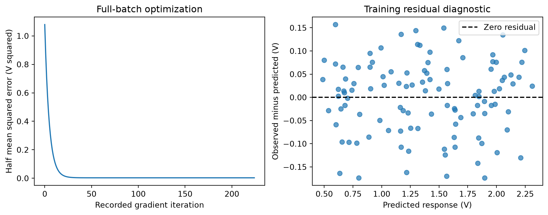
A residual plot can reveal patterns hidden by an average metric. We inspect training residuals for development diagnostics, rather than using test residuals to choose a new model after the final evaluation. A curved pattern suggests a missing nonlinear term; a widening band suggests changing error variance. A finite plot cannot prove independence, normality, or correct specification.
# Step 8: Plot numerical convergence and training residual structure.# Residuals use observed minus predicted response, in volts.training_predictions = training_design @ scratch_parameterstraining_residuals = training_targets - training_predictions# Two panels separate the numerical objective from model diagnostics.figure, axes = plt.subplots(1, 2, figsize=(10, 4))axes[0].plot(scratch_loss_history)axes[0].set_title("Full-batch optimization")axes[0].set_xlabel("Recorded gradient iteration")axes[0].set_ylabel("Half mean squared error (V squared)")axes[1].scatter(training_predictions, training_residuals, alpha=0.7)axes[1].axhline(0.0, color="black", linestyle="--", label="Zero residual")axes[1].set_title("Training residual diagnostic")axes[1].set_xlabel("Predicted response (V)")axes[1].set_ylabel("Observed minus predicted (V)")axes[1].legend()figure.tight_layout()plt.show()
Figure 14.1: Synthetic calibration: training-objective convergence and observed-minus-predicted training residuals. These are development diagnostics, not a test-set model-selection step.
14.8.3 Experiment 3: Change only the learning rate
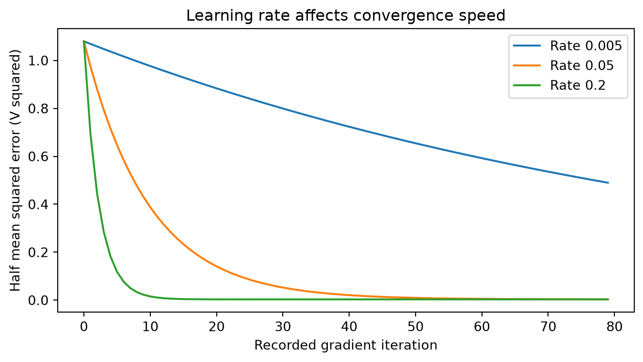
Question: how quickly do several stable rates approach the same optimum? Hold the data, initialization, gradient, and 80-update budget fixed. This is a numerical experiment using training loss, not model selection on test targets. A smaller loss after a fixed number of updates means faster progress in this example; it does not make the resulting model family more expressive.
# Step 9: Compare rates under the same short optimization budget.# These rates are explicit experiment settings, not universal recommendations.learning_rates = [0.005, 0.05, 0.2]# Store the actual final objective for each run.rate_results = []# One plot shows the full path rather than only its final point.figure, axis = plt.subplots(figsize=(7, 4))for current_rate in learning_rates:# Disable early stopping to compare the same update budget. rate_parameters, rate_losses = fit_gradient_descent( training_design, training_targets, learning_rate=current_rate, maximum_iterations=80, gradient_tolerance=0.0 )# Evaluate after the last update; history records pre-update losses. final_rate_errors = training_design @ rate_parameters - training_targets final_rate_loss = np.mean(final_rate_errors **2) /2 rate_results.append({"Learning rate": current_rate, "Final half-MSE (V squared)": final_rate_loss}) axis.plot(rate_losses, label=f"Rate {current_rate}")axis.set_title("Learning rate affects convergence speed")axis.set_xlabel("Recorded gradient iteration")axis.set_ylabel("Half mean squared error (V squared)")axis.legend()figure.tight_layout()plt.show()print(pd.DataFrame(rate_results).to_string(index=False))
Figure 14.2: Learning-rate comparison on the same standardized synthetic training data. Initialization and the 80-update budget are held fixed.
 Learning rate  Final half-MSE (V squared)
         0.005                    0.484950
         0.050                    0.003364
         0.200                    0.003072
Too large a rate can oscillate or diverge; too small a rate may leave substantial optimization error. The main fitted model already passed a gradient check, so these short-run differences do not invalidate its agreement with least squares.
14.8.4 Experiment 4: Polynomial features and validation selection
Linear in parameters does not require a straight line in the raw input. With a scalar input \(x\), the model \(b+w_1x+w_2x^2\) remains linear in its coefficients. Polynomial expansion changes the design columns. It can represent curvature but can also amplify numerical problems and extrapolation error.
Use a second, independent synthetic development problem. Its target is an invented quadratic response, without physical units. We compare degrees 1, 2, and 8 on a training/validation split. This experiment does not access the calibration test set and does not report a final generalization estimate for a selected polynomial model.
# Step 10: Compare polynomial degrees using independent validation data.from sklearn.preprocessing import PolynomialFeatures# A separate generator keeps this experiment independent of calibration data.polynomial_generator = np.random.default_rng(73)# Dimensionless scalar inputs are stored as a one-column feature matrix.polynomial_features = polynomial_generator.uniform(-2.0, 2.0, (70, 1))# The target combines known curvature with zero-mean noise.polynomial_targets = (1.0+0.5* polynomial_features[:, 0]+0.8* polynomial_features[:, 0] **2+ polynomial_generator.normal(0.0, 0.35, 70))# Validation rows are held apart before fitting expansion/scaling/model steps.poly_training_features, poly_validation_features, poly_training_targets, poly_validation_targets = train_test_split( polynomial_features, polynomial_targets, test_size=0.30, random_state=42)# Each candidate changes only degree; partitions and estimator remain aligned.polynomial_rows = []for current_degree in [1, 2, 8]:# Avoid duplicate intercept columns by excluding the expansion's bias term. polynomial_model = Pipeline([ ("polynomial", PolynomialFeatures(degree=current_degree, include_bias=False)), ("scaler", StandardScaler(with_mean=True, with_std=True)), ("regression", LinearRegression(fit_intercept=True)), ]) polynomial_model.fit(poly_training_features, poly_training_targets)# Evaluate training fit and separate validation error for the same candidate. poly_training_predictions = polynomial_model.predict(poly_training_features) poly_validation_predictions = polynomial_model.predict(poly_validation_features) polynomial_rows.append({"Degree": current_degree,"Training RMSE": root_mean_squared_error(poly_training_targets, poly_training_predictions),"Validation RMSE": root_mean_squared_error(poly_validation_targets, poly_validation_predictions), })# The lowest validation error nominates a degree for later evaluation.polynomial_results = pd.DataFrame(polynomial_rows)best_degree_row = polynomial_results["Validation RMSE"].idxmin()selected_degree =int(polynomial_results.loc[best_degree_row, "Degree"])print(polynomial_results.to_string(index=False))print("Degree selected on this validation split:", selected_degree)
 Degree  Training RMSE  Validation RMSE
      1       1.020206         1.116728
      2       0.367149         0.384201
      8       0.320219         0.375719
Degree selected on this validation split: 8
Read the measured validation results before deciding whether the most flexible candidate helps. The true generator being quadratic does not guarantee degree two wins every finite noisy split. More candidate searches can overfit validation too; repeated or nested evaluation is needed for stronger comparisons. The polynomial feature API documents the expansion settings.
14.9 Assumptions and hyperparameters
Separate the assumptions required to calculate a fit, to interpret coefficients, and to infer uncertainty:
Item
Why it matters
Practical check or response
Numeric finite inputs and matched rows
The computation requires well-defined arithmetic.
Audit shape, missingness, units, and identifiers.
Additive linear conditional mean in chosen features
Supports interpreting the fitted relationship as a conditional mean model.
Inspect residual patterns; consider justified interactions or transformations.
Supports unbiased coefficients under the linear model and fixed/full-rank design conditions.
Investigate omitted confounders and measurement processes; residual plots alone cannot verify it.
Suitable independence and stable deployment sampling
Supports the intended validation and classical uncertainty statements.
Use groups/time-aware splits and investigate distribution shift.
Equal conditional error variance
Needed for the usual constant-variance OLS standard-error formula, not to calculate the fit.
Inspect variance patterns; use appropriate inference methods if needed.
Gaussian errors
Supports exact normal-theory small-sample inference under the remaining conditions.
Do not infer it from the fitting procedure.
OLS has no regularization-strength hyperparameter. Whether to include an intercept and which features or polynomial degree to use change the model specification. Gradient-descent learning rate, tolerance, and iteration limit control numerical optimization; they do not add model flexibility. Scaling aids numerical optimization but does not automatically cure near dependence. LinearRegression’s positive option changes the feasible coefficient set and is therefore a different constrained model.
If \(A\) has full column rank, \(E[\boldsymbol\varepsilon\mid A]=\mathbf0\), and \(\operatorname{Cov}(\boldsymbol\varepsilon\mid A)=\sigma^2I\), then
To see the source of this expression, substitute \(\mathbf y=A\boldsymbol\theta+\boldsymbol\varepsilon\) into the solution. The estimation error is \((A^TA)^{-1}A^T\boldsymbol\varepsilon\). Multiplying its covariance on both sides and using \(\operatorname{Cov}(\boldsymbol\varepsilon\mid A)=\sigma^2I\) gives the expression. Nearly dependent columns can make this covariance large. A residual standard-deviation estimate is \(\hat\sigma=\sqrt{\mathrm{SSE}/(n-p-1)}\) when \(n>p+1\) and all \(p+1\) parameters are identifiable. An interval for the mean response and an interval for a new noisy observation are different: the latter also includes new-observation noise. We do not attach inferential intervals to the synthetic coefficient table merely because a library returns coefficients.
14.10 Advantages, limitations, and failure modes
Advantages: few parameters, fast prediction, explicit unit-aware coefficients, and a strong auditable baseline for continuous targets. An inspectable model is valuable even when another model later predicts better.
Curvature: residuals that vary systematically with inputs suggest that the selected features omit structure. Add justified transformations or consider a different family; do not keep increasing polynomial degree against test results.
Outliers and leverage: a large response error receives a squared penalty. A row far from the feature cloud has high leverage and can greatly affect coefficients. Verify data provenance before deleting it. Compare sensitivity with and without a documented questionable row, using development data.
Multicollinearity: two almost duplicate sensors can produce unstable slopes while predictions remain adequate within the observed feature combinations. Coefficient instability is not fixed by printing more decimal places.
Extrapolation: a line continues indefinitely and a polynomial may grow rapidly. Prediction accuracy inside a calibration range does not validate values outside it.
Dependence and shift: repeated windows from a participant are not independent new people. Randomly splitting such windows can overstate generalization.
Interpretation: a coefficient is an association conditional on included features, their encoding, and the training distribution. It is not automatically a causal effect or a clinical finding.
Common implementation errors are forgetting the intercept, updating the intercept with the wrong gradient, mixing residual sign conventions, scaling with test rows, leaving targets with shape \((n,1)\) so subtraction broadcasts to \((n,n)\), and comparing standardized coefficients with original-unit generating coefficients.
14.11 Computational and memory complexity
Let \(n\) be training rows, \(p\) raw features, \(d=p+1\) design columns including the intercept, \(T\) full-batch updates, and \(m\) new observations. For dense arrays:
Operation
Time
Additional context
Training scaling
\(O(np)\)
Stores \(O(p)\) statistics; a copied transformed dataset needs \(O(np)\) memory.
Full-batch gradient descent
\(O(Tnd)\)
Each update computes predictions and a gradient. The educational parameter loop preserves this order.
Dense QR/SVD-style least squares, \(n\geq d\)
Typically \(O(nd^2)\)
Solver and matrix shape matter; wide systems need a different shape-aware expression.
Prediction
\(O(md)\)
Model parameters occupy \(O(d)\) storage.
The scratch code stores the dense design matrix in \(O(nd)\) space, error/prediction vectors in \(O(n)\), parameters/gradient in \(O(d)\), and loss history in \(O(T)\). Avoiding history reduces that term. These are storage orders, not measured memory consumption. Forming normal equations would require an additional \(O(d^2)\) matrix and can worsen numerical stability. With \(p\) raw features and total polynomial degree \(k\), the full polynomial expansion has \(\binom{p+k}{k}\) columns including the constant. Complexity must use that expanded column count. This is why polynomial regression can cease to be a small problem.
14.12 Comparison with related algorithms
Method
What changes from OLS
Reason to consider it
Training-mean predictor
Ignores features.
Minimum baseline for checking whether inputs help.
Polynomial regression
Expands features; remains linear in parameters.
Smooth nonlinear relationships with a controlled low-degree basis.
Ridge/Lasso
Adds a coefficient penalty.
Later tools for variance control or sparsity; penalty tuning requires validation.
Logistic regression
Models class probabilities using a different objective and link.
Categorical targets; continuous OLS predictions are not class probabilities.
Neighbor or tree regression
Replaces a global additive linear surface with local structure.
Later alternatives for interactions and nonlinear behavior, with different costs and failure modes.
These are choices for different data and tasks. Logistic regression is the next teaching chapter because it extends the supervised workflow to classification, not because it universally supersedes continuous-target regression.
14.13 Applications and selection guidance
Choose linear regression when the target is continuous, a global additive approximation is plausible in the intended operating range, the feature count is manageable, and you need an understandable baseline. Calibration, limited-range trend prediction, and relating engineered sensor summaries to a continuous response are useful educational settings. Check units and sampling before choosing the estimator.
Define the deployment unit and information available when a prediction is made.
Establish a mean baseline and a valid split before fitting anything learned.
Fit a simple intercept model and inspect errors on development data.
Investigate unexpected residual structure, feature dependence, and implausible coefficients.
Consider transformations, regularization, or another family using validation.
Evaluate the fixed final procedure on an appropriate untouched test set.
Do not use the calibration experiment as evidence that an actual sensor follows this law. For gait research, predicting a continuous laboratory measurement and diagnosing a clinical condition are distinct tasks, with distinct labels and evidence requirements.
14.14 Interview questions and exercises
14.14.1 Questions
Why do we average squared errors instead of summing signed residuals? Does the factor \(1/(2n)\) change the minimizer?
For the three-point example, verify the residual sum and MSE. What would the best intercept-only predictor be?
Starting from \(J\), derive the intercept update and explain the error sign used in the code.
Is \(b+w_1x+w_2x^2\) linear regression? Can a unique coefficient vector exist when two design columns are identical?
Does a negative test \(R^2\) prove the optimization failed? Explain which comparison is in its denominator.
Why can coefficients vary sharply between resamples while in-range predictions barely change?
Modify the synthetic calibration force feature to be measured in kilonewtons. What happens to its coefficient and to predictions if the model is fitted consistently?
A dataset has 30 windows per participant. Deployment is to unseen participants. What split should replace the random row split?
Implement a central-difference gradient check on five training rows. Compare each analytic component with a finite difference using \(h=10^{-6}\).
On a separate development-only experiment, introduce one large response error. Compare coefficient changes. Explain why blindly removing the row would be scientifically unsafe.
14.14.2 Worked answers
Signed errors can cancel even when individual predictions are poor. A positive constant multiplier does not change an objective’s minimizer, although it scales its derivative and therefore affects a fixed learning rate.
Residuals are \(-1/6,1/3,-1/6\), which sum to zero. Their squared sum is \(1/6\) and MSE is \(1/18\). The intercept-only fit predicts \(5/3\) for every row; its MSE is \(2/9\), larger here.
Because \(\partial\hat y_i/\partial b=1\), \(\partial J/\partial b=\frac1n\sum_i(\hat y_i-y_i)\). Subtract this gradient times the rate. If residuals were instead observed minus predicted, the equivalent update would add their mean times the rate.
Yes: its unknown coefficients enter linearly. Duplicate columns make the design rank deficient, so multiple coefficient vectors give the same fitted values. A solver’s chosen solution does not restore identifiability.
No. It means squared error exceeds the error of predicting the evaluation set’s mean for every evaluation observation. Poor specification, shift, a small noisy test set, or numerical failure are possible explanations; inspect evidence rather than assuming one.
Nearly dependent features make individual effects hard to distinguish. Different large coefficients may compensate on the observed combinations but disagree strongly under extrapolation.
A kilonewton equals 1000 N, so the corresponding numerical slope is 1000 times larger in V/kN. Consistently converted predictions remain the same, apart from numerical roundoff.
Hold complete participants apart. Tune with group-aware folds inside the development participants and reserve test participants. If deployment also concerns future time, the split must respect that timing too.
A runnable check follows. It checks a nonzero parameter vector so a zero-initialization special case cannot conceal a mistake.
# Exercise 9 solution: compare analytic and central-difference gradients.# A small subset keeps every calculation easy to inspect.check_design = training_design[:5]check_targets = training_targets[:5]# Arbitrary nonzero coefficients, unrelated to the fitted optimum.check_parameters = np.array([0.3, -0.2, 0.1])# Analytic gradient uses exactly the chapter's loss normalization.analytic_gradient = check_design.T @ (check_design @ check_parameters - check_targets) /len(check_targets)# Perturbation balances truncation and floating-point effects in this example.difference_step =1e-6# Store one numerical derivative for each parameter.numerical_gradient = np.zeros(len(check_parameters))for parameter_index inrange(len(check_parameters)):# Independent copies perturb only the selected coordinate. plus_parameters = check_parameters.copy() minus_parameters = check_parameters.copy() plus_parameters[parameter_index] += difference_step minus_parameters[parameter_index] -= difference_step# Calculate the same half-MSE for both nearby parameter vectors. plus_loss = np.mean((check_design @ plus_parameters - check_targets) **2) /2 minus_loss = np.mean((check_design @ minus_parameters - check_targets) **2) /2 numerical_gradient[parameter_index] = (plus_loss - minus_loss) / (2* difference_step)print("Largest gradient-check discrepancy:", np.max(np.abs(analytic_gradient - numerical_gradient)))assert np.allclose(analytic_gradient, numerical_gradient, atol=1e-8, rtol=1e-6)
Largest gradient-check discrepancy: 1.1051409787299349e-10
For a concrete development-only sensitivity calculation, add 3 V to the first training target. Keeping features and all other targets fixed isolates the response perturbation. The resulting coefficients are computed below. Squared loss makes a large error influential, but the row could represent a true operating condition; investigate provenance and document any exclusion rule before evaluating on test data.
# Exercise 10 solution: measure sensitivity using training rows only.# Copy targets so the main experiment's data and scores remain intact.perturbed_training_targets = training_targets.copy()# Add a deliberately large synthetic response error to one training row.perturbed_training_targets[0] +=3.0# Fit the same numerical problem after changing only that response.perturbed_parameters = np.linalg.lstsq(training_design, perturbed_training_targets, rcond=None)[0]# Difference quantifies coefficient sensitivity in standardized feature units.parameter_change = perturbed_parameters - direct_parametersprint("Change [intercept, force slope, temperature slope]:", parameter_change)
Change [intercept, force slope, temperature slope]: [0.02777778 0.02521013 0.00242816]
14.15 One-page revision summary
Item
Remember
Task
Predict a continuous target using a weighted sum of chosen features and an intercept.
Prediction
\(\hat{\mathbf y}=A\boldsymbol\theta\), with \(A\) shaped \(n\times(p+1)\).
Objective
\(J=\|A\boldsymbol\theta-\mathbf y\|^2/(2n)\); MSE is \(2J\).
Gradient
\(A^T(A\boldsymbol\theta-\mathbf y)/n\); update by subtraction.
Stationary equation
\(A^TA\hat{\boldsymbol\theta}=A^T\mathbf y\); unique coefficients require full column rank.
Numerical practice
Prefer QR/SVD least-squares solves to an explicit inverse; verify descent convergence.
Preprocessing
Fit training means/scales only; preserve row order and feature meaning.
Evaluation
Compare with a training-mean baseline; tune on validation; reserve test for the fixed procedure.
Units
Slope units are target units divided by feature units. Undo scaling before interpreting original units.
Main risks
Curvature, outliers, multicollinearity, extrapolation, dependence, leakage, and causal overinterpretation.
Costs
Dense gradient descent \(O(Tnp)\); common tall-matrix direct solves \(O(np^2)\), using expanded feature count if applicable.
Next question
How should predictions and loss change for a categorical target? This motivates Logistic Regression.
14.16 Sources and further reading
An Introduction to Statistical Learning, official author site: the linear-regression chapter develops fitting, diagnostics, and interpretation. The derivations and synthetic experiments here are worked explicitly so they can be checked independently.