10 Numerical optimization

10.1 Turning a loss into fitted parameters

A mathematical objective tells us which parameter values we prefer. An optimization algorithm tells us how to search for them. These are different parts of a learning system. The same objective may be minimized with a direct linear-algebra solver or an iterative method, and an optimizer can only optimize the objective it is given. A wrong target, leakage, or an inappropriate loss is not repaired by a lower training error.

This chapter implements a complete small gradient-descent procedure for mean squared error. We explain learning rates, curvature, stopping, numerical checks, and constraints. We also distinguish optimization progress on fixed training data from generalization to future observations. Our synthetic example compares numerical fitting methods on one fixed problem; it is not a model-selection experiment or a claim about test performance.

Prerequisites: vector and matrix products from Chapter 6 and gradients, Hessians, and finite differences from Chapter 9. Familiarity with train/validation/test separation will be developed in the workflow chapters before the complete regression experiment.

Learning objectives:

Distinguish an objective, parameters, and optimization settings.
Derive and implement a full-batch gradient-descent update.
Relate learning-rate stability to the curvature of a quadratic.
Use meaningful stopping criteria and interpret failure to converge.
Compare an iterative fit with a direct least-squares solution and explain constraints.

10.2 Define the problem before choosing the optimizer

Write a minimization problem as

\[ \operatorname*{minimize}_{\boldsymbol\beta\in\mathcal C} J(\boldsymbol\beta). \]

The vector \(\boldsymbol\beta\in\mathbb R^d\) contains the unknown parameters, \(J\) is a scalar objective, and \(\mathcal C\) is the feasible set of allowed parameter values. If \(\mathcal C=\mathbb R^d\), the problem is unconstrained. A nonnegative-coefficient requirement, a fixed parameter sum, or a norm limit makes it constrained. A constraint should reflect a justified modeling decision, not be added solely to force a preferred numerical result.

The loss function often measures one observation’s prediction error. The training objective aggregates such losses and may add a regularization penalty. For example, \(J(\boldsymbol\beta)=n^{-1}\sum_i\ell_i(\boldsymbol\beta) +\lambda R(\boldsymbol\beta)\), where \(\lambda\geq0\) controls the penalty strength and \(R\) penalizes selected parameter configurations. Changing the penalty changes the optimization problem and potentially the fitted model, not merely the path taken to the same answer.

The learning rate and iteration limit are settings of the optimizer. They control how it searches. Model settings and optimizer settings can interact: poor optimization may make a model look weak even when its objective has not been adequately minimized. Conversely, fully minimizing training loss does not guarantee useful predictions on new data.

10.3 Gradient descent from the local approximation

For a differentiable objective, a small displacement \(\Delta\) gives \(J(\boldsymbol\beta+\Delta)\approx J(\boldsymbol\beta)+\nabla J(\boldsymbol\beta)^\top\Delta\). Choose \(\Delta=-\eta\nabla J(\boldsymbol\beta)\) with \(\eta>0\). The approximate change becomes

\[ -\eta\|\nabla J(\boldsymbol\beta)\|_2^2\leq0. \]

This suggests the gradient-descent update

\[ \boldsymbol\beta^{(t+1)} =\boldsymbol\beta^{(t)}-\eta\nabla J(\boldsymbol\beta^{(t)}). \]

The superscript \((t)\) labels an iteration, not exponentiation. The learning rate \(\eta\) scales the step. The approximation explains why a sufficiently small local step often decreases loss. It does not prove that any positive learning rate will work or that every stationary point is a global minimum. The coordinate units and the objective’s normalization also affect the meaning of the numerical learning rate.

For the dimensionless scalar objective \(J(w)=(w-3)^2\), the derivative is \(2(w-3)\). Starting from \(w^{(0)}=0\) with \(\eta=0.1\) gives \(w^{(1)}=0-0.1[-6]=0.6\). The loss falls from 9 to \(2.4^2=5.76\). The next derivative is \(-4.8\), so \(w^{(2)}=1.08\). Recomputing the gradient at each new location matters: repeatedly applying the initial gradient would not be gradient descent.

10.3.1 Conceptual procedure

Define a complete objective and its gradient using the same normalization.
Choose an initial parameter vector and optimizer settings.
Evaluate predictions, loss, and the gradient at the current parameters.
Stop if a justified convergence criterion is met.
Subtract the scaled gradient from every parameter simultaneously.
Check finite values and record progress; repeat until convergence or a limit.

Simultaneous updating means computing the whole gradient from the old parameter vector before changing coordinates. Updating one parameter and using that new value to calculate another coordinate’s gradient defines a different procedure.

10.4 Convexity and what convergence can establish

A set is convex if the line segment between any two feasible points stays in the set. A function on a convex domain is convex if

\[ J(\tau\mathbf a+(1-\tau)\mathbf b) \leq\tau J(\mathbf a)+(1-\tau)J(\mathbf b), \quad 0\leq\tau\leq1. \]

Geometrically, the graph lies at or below each chord. A differentiable convex function has the useful first-order property \(J(\mathbf b)\geq J(\mathbf a)+\nabla J(\mathbf a)^\top(\mathbf b-\mathbf a)\). Consequently, an unconstrained stationary point is a global minimizer. A strictly convex objective has at most one minimizer on a convex domain. Convexity alone does not guarantee a minimizer exists; for example, \(e^w\) approaches zero as \(w\to-\infty\) but never attains zero.

For a twice differentiable objective on an open convex domain, a positive semidefinite Hessian everywhere characterizes convexity. Linear-model MSE has \(H=(2/n)D^\top D\succeq0\), so it is convex. If \(D\) has full column rank, this quadratic is strictly convex and has one minimizer. With redundant columns, several coefficient vectors can minimize the same objective.

For a nonconvex objective, a small gradient may occur near a local minimum, a saddle, or a flat region. An optimizer’s success flag then does not prove global optimality. Even for a convex problem, practical convergence depends on appropriate step choices, numerical behavior, and a sufficient stopping budget. Boyd and Vandenberghe’s Convex Optimization is a primary reference for these distinctions and the wider theory.

10.5 Learning rate and curvature: an exact stability calculation

Consider \(J(w)=\tfrac12a(w-w_*)^2\) with curvature \(a>0\) and minimizer \(w_*\). Define the parameter error \(e_t=w^{(t)}-w_*\). Gradient descent gives

\[ e_{t+1}=(1-\eta a)e_t, \qquad e_t=(1-\eta a)^t e_0. \]

The error converges to zero when \(|1-\eta a|<1\), equivalently \(0<\eta<2/a\). If \(0<\eta a<1\), the error shrinks without changing sign. If \(1<\eta a<2\), it alternates signs while shrinking. At \(\eta a=2\) it oscillates without shrinking, and above that value its magnitude grows. A very small learning rate is stable but can be slow.

For \(J(w)=(w-3)^2\), \(a=2\), so the stable interval is \(0<\eta<1\). This result applies exactly to this scalar quadratic. It is not a universal numerical range for every machine-learning objective.

For a positive-definite quadratic with Hessian \(H\), each eigenvector direction behaves like a scalar quadratic with curvature equal to its eigenvalue. A sufficient and necessary fixed-step stability range for all directions is \(0<\eta<2/\lambda_{\max}(H)\). Very different eigenvalues create a narrow, elongated valley: the largest curvature limits the step while small-curvature directions progress slowly. Feature scaling can improve this geometry, but any scaling learned from data must be fitted only on training data in an evaluated predictive workflow.

10.5.1 A learning-rate experiment with known answers

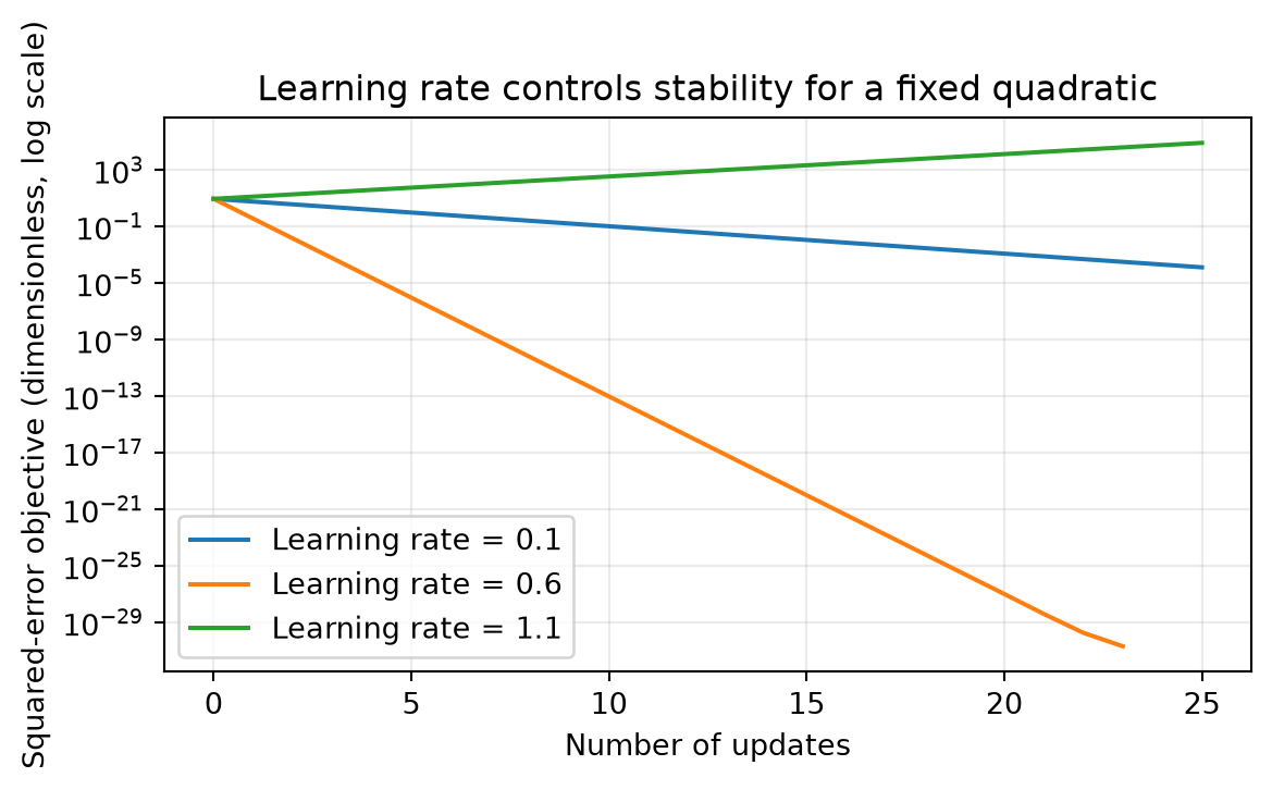
Only the learning rate changes; the objective, initial value, and number of updates remain fixed. We compare a small stable step, an oscillating stable step, and a step beyond the stability boundary. There is no randomness.

# Step 1: Import the numerical and plotting tools for this independent chapter.
import numpy as np
import matplotlib.pyplot as plt

# Step 2: Set controlled conditions for the scalar quadratic experiment.
# Each run starts at zero, while the exact minimizer is three.
initial_weight = 0.0
# Twenty-five updates make the different paths visible without expensive computation.
number_of_updates = 25
# The stability boundary is one for this objective's curvature of two.
learning_rates = [0.1, 0.6, 1.1]

# Step 3: Record each path's loss after every simultaneous scalar update.
figure, axis = plt.subplots(figsize=(6.2, 3.6))
for learning_rate in learning_rates:
    # Reset the parameter so the comparison isolates the learning rate.
    current_weight = initial_weight
    # Include the initial loss at update zero.
    scalar_loss_history = [(current_weight - 3.0) ** 2]
    for update_index in range(number_of_updates):
        # This derivative is recalculated at the current parameter value.
        current_derivative = 2.0 * (current_weight - 3.0)
        # Subtracting the gradient seeks a lower local objective value.
        current_weight = current_weight - learning_rate * current_derivative
        scalar_loss_history.append((current_weight - 3.0) ** 2)
    # A logarithmic axis cannot display exact zero; retain only positive history entries.
    # A fast-converging path can reach the exactly represented minimizer through rounding.
    scalar_loss_values = np.array(scalar_loss_history)
    update_numbers = np.arange(len(scalar_loss_values))
    positive_loss_mask = scalar_loss_values > 0.0
    axis.semilogy(
        update_numbers[positive_loss_mask],
        scalar_loss_values[positive_loss_mask],
        label=f"Learning rate = {learning_rate}"
    )
    print("Learning rate:", learning_rate, "Final loss:", scalar_loss_history[-1])

# Step 4: Use a logarithmic loss axis to compare decreasing and increasing paths.
axis.set_xlabel("Number of updates")
axis.set_ylabel("Squared-error objective (dimensionless, log scale)")
axis.set_title("Learning rate controls stability for a fixed quadratic")
axis.legend()
axis.grid(alpha=0.25)
figure.tight_layout()
plt.show()

Learning rate: 0.1 Final loss: 0.00012845229234353253
Learning rate: 0.6 Final loss: 0.0
Learning rate: 1.1 Final loss: 81903.94335001991

Figure 10.1: Gradient descent on a fixed scalar quadratic: only the learning rate changes. Exact-zero rounded losses are excluded from the logarithmic display.

The stable oscillation concerns parameter values around the optimum, not a requirement that the loss itself oscillate. For this quadratic, squared error decreases geometrically whenever the error multiplier has magnitude below one. The deliberately unstable run demonstrates a known failure mode rather than a hyperparameter search on held-out data.

The fast stable run can round to the exactly representable minimizer, producing a stored loss of zero. The plot omits those zero entries because a logarithmic axis cannot display them; the printed final loss retains the actual value. This is finite-precision behavior, while the geometric convergence derivation describes exact arithmetic.

10.6 A complete full-batch MSE implementation

For \(D\in\mathbb R^{n\times d}\), targets \(\mathbf y\in\mathbb R^n\), and coefficients \(\boldsymbol\beta\in\mathbb R^d\), use

\[ J(\boldsymbol\beta)=\frac1n\|D\boldsymbol\beta-\mathbf y\|_2^2, \qquad \nabla J=\frac2nD^\top(D\boldsymbol\beta-\mathbf y). \]

This is full-batch gradient descent because every gradient uses all observations. The implementation is educational: it stores a loss history and uses a fixed learning rate. It does not include line search, automatic scaling, momentum, adaptive learning rates, or support for sparse matrices. The calculations remain explicit enough to connect with the equations.

We stop when the gradient norm falls below a specified tolerance, or when an iteration cap is reached. These outcomes are returned separately. A limit is a safeguard on computation, not evidence of convergence. Nonfinite numerical values also produce a distinct status so a failed run cannot silently appear successful.

# Step 5: Define the objective and gradient together to keep their normalization aligned.
def mse_value_and_gradient(coefficients, design_matrix, targets):
    """Return MSE and its gradient for finite dense arrays.

    coefficients has shape (d,), design_matrix has shape (n, d), and
    targets has shape (n,). The loss is in squared target units;
    each gradient entry is loss units divided by its coefficient's unit.
    """
    # Produce one prediction per observation before measuring the errors.
    predicted_targets = design_matrix @ coefficients
    # Keep the predicted-minus-observed convention used by the gradient derivation.
    prediction_errors = predicted_targets - targets
    # Average squared errors so the loss does not simply grow with row count.
    objective_value = float(np.mean(prediction_errors ** 2))
    # Accumulate feature-weighted errors for every coefficient.
    gradient = 2.0 * design_matrix.T @ prediction_errors / len(targets)
    return objective_value, gradient

# Step 6: Implement explicit iterative updates and report the actual stopping reason.
def fit_mse_gradient_descent(
    design_matrix,
    targets,
    initial_coefficients,
    learning_rate,
    maximum_iterations=2000,
    gradient_tolerance=1e-8
):
    """Fit a small dense least-squares problem by full-batch gradient descent.

    design_matrix is (n, d), targets is (n,), and initial_coefficients is (d,).
    Arrays must be finite, n must be positive, and learning_rate must be positive.
    maximum_iterations caps updates; gradient_tolerance is nonnegative.
    Returns a dictionary containing coefficients, loss_history, update_count,
    final_gradient_norm, and status. A maximum-iteration status is not convergence.
    """
    # Check shape conventions before any broadcasting or matrix multiplication occurs.
    if design_matrix.ndim != 2 or targets.ndim != 1:
        raise ValueError("Use a two-dimensional design and one-dimensional targets.")
    if design_matrix.shape[0] != len(targets) or len(targets) == 0:
        raise ValueError("The design and nonempty targets must have the same row count.")
    if initial_coefficients.shape != (design_matrix.shape[1],):
        raise ValueError("There must be one initial coefficient per design column.")
    if learning_rate <= 0.0 or maximum_iterations < 1 or gradient_tolerance < 0.0:
        raise ValueError("Use a positive rate and iteration count, and a nonnegative tolerance.")
    if not np.all(np.isfinite(design_matrix)) or not np.all(np.isfinite(targets)):
        raise ValueError("Design and targets must be finite.")
    if not np.all(np.isfinite(initial_coefficients)):
        raise ValueError("Initial coefficients must be finite.")

    # Copy the initial values so fitting does not mutate the caller's array.
    coefficients = initial_coefficients.astype(float).copy()
    # Record the starting loss before performing any update.
    initial_loss, initial_gradient = mse_value_and_gradient(coefficients, design_matrix, targets)
    # The history includes update zero for a complete progress trace.
    loss_history = [initial_loss]
    # Preserve a distinct default status if the update budget is exhausted.
    status = "maximum_iterations_reached"

    # Step 7: Calculate each new vector from the entire old coefficient vector.
    for iteration_index in range(maximum_iterations):
        # Evaluate the current point rather than reusing a stale derivative.
        current_loss, current_gradient = mse_value_and_gradient(coefficients, design_matrix, targets)
        # A small norm means all coordinate derivatives are collectively small in this scaling.
        current_gradient_norm = np.linalg.norm(current_gradient)
        if not np.isfinite(current_loss) or not np.isfinite(current_gradient_norm):
            status = "nonfinite_calculation"
            break
        if current_gradient_norm <= gradient_tolerance:
            status = "gradient_tolerance_reached"
            break

        # Construct a candidate vector before replacing the old vector.
        candidate_coefficients = coefficients - learning_rate * current_gradient
        # Evaluate the candidate so numerical failure is checked before acceptance.
        candidate_loss, candidate_gradient = mse_value_and_gradient(
            candidate_coefficients, design_matrix, targets
        )
        if not np.isfinite(candidate_loss) or not np.all(np.isfinite(candidate_gradient)):
            status = "nonfinite_calculation"
            break
        # Accept the complete simultaneous update and append its actual loss.
        coefficients = candidate_coefficients
        loss_history.append(candidate_loss)

    # Step 8: Report the quality of the returned point, including a final accepted update.
    final_loss, final_gradient = mse_value_and_gradient(coefficients, design_matrix, targets)
    # The final norm may meet tolerance on the very last allowed update.
    final_gradient_norm = float(np.linalg.norm(final_gradient))
    if np.isfinite(final_gradient_norm) and final_gradient_norm <= gradient_tolerance:
        status = "gradient_tolerance_reached"
    return {
        "coefficients": coefficients,
        "loss_history": np.array(loss_history),
        "update_count": len(loss_history) - 1,
        "final_gradient_norm": final_gradient_norm,
        "status": status
    }

The tolerance is expressed in this particular parameterization. An absolute gradient threshold suitable for dimensionless order-one data may be unsuitable for a differently scaled problem. The implementation detects nonfinite arithmetic but does not automatically rescue an excessive learning rate. Inspection and an informed change of settings remain necessary.

10.6.1 Fit a reproducible artificial problem

We generate 21 inputs over \([-1,1]\), then targets from a straight line plus small normal noise. The generating coefficients are known because this is a simulation. Noise means the best coefficients for the finite sample need not equal those generating values exactly. The correct numerical reference is the least-squares optimum for these same observed targets.

# Step 9: Construct a complete synthetic problem without external data.
# A fixed seed makes this numerical comparison reproducible within the software setup.
random_generator = np.random.default_rng(42)
# Symmetric, dimensionless inputs keep the intercept and slope geometry easy to inspect.
input_values = np.linspace(-1.0, 1.0, 21)
# Each row contains the intercept multiplier and the observation's input value.
design_matrix = np.column_stack((np.ones(len(input_values)), input_values))
# The known generating intercept and slope define the artificial mean relationship.
generating_coefficients = np.array([2.0, 3.0])
# Independent normal noise has standard deviation 0.15 in dimensionless target units.
target_noise = random_generator.normal(loc=0.0, scale=0.15, size=len(input_values))
# These noisy observations are fixed for every solver comparison below.
observed_targets = design_matrix @ generating_coefficients + target_noise

# Step 10: Choose a learning rate using this quadratic's largest curvature.
# The MSE Hessian is constant for this fixed design.
objective_hessian = 2.0 * design_matrix.T @ design_matrix / len(observed_targets)
# eigvalsh returns ordered eigenvalues for the symmetric Hessian.
hessian_eigenvalues = np.linalg.eigvalsh(objective_hessian)
# The upper stability boundary is 2 / largest_eigenvalue for this positive-definite quadratic.
stability_boundary = 2.0 / hessian_eigenvalues[-1]
# Pick a conservative rate inside that verified interval rather than guessing a universal default.
learning_rate = 0.2
assert 0.0 < learning_rate < stability_boundary

# Step 11: Fit from zero coefficients and preserve the actual status and history.
fitting_result = fit_mse_gradient_descent(
    design_matrix,
    observed_targets,
    initial_coefficients=np.zeros(design_matrix.shape[1]),
    learning_rate=learning_rate,
    maximum_iterations=2000,
    gradient_tolerance=1e-8
)
print("Stopping status:", fitting_result["status"])
print("Updates:", fitting_result["update_count"])
print("Final gradient norm:", fitting_result["final_gradient_norm"])
print("Estimated intercept and slope:", fitting_result["coefficients"])
assert fitting_result["status"] == "gradient_tolerance_reached"

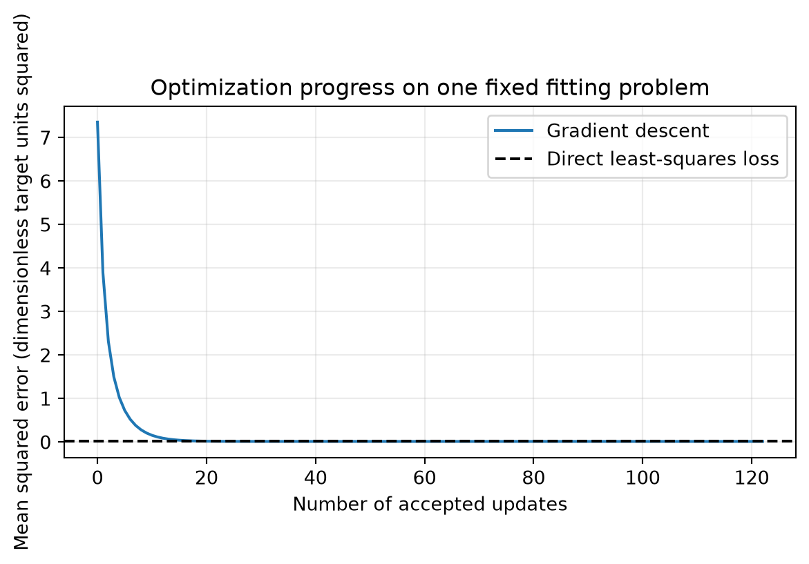
Stopping status: gradient_tolerance_reached
Updates: 122
Final gradient norm: 8.77437039163775e-09
Estimated intercept and slope: [1.99397497 3.02992473]

The result reports how the numerical search ended. A lower loss alone would not establish convergence; the returned gradient norm and the known convex geometry make the conclusion more specific. This optimization diagnostic uses the fitting data throughout and does not estimate out-of-sample prediction error.

10.7 Compare with a library least-squares solver

A dense direct least-squares solver solves this small linear problem without gradient-descent iterations. Using it provides an independent implementation check and illustrates that gradient descent is a choice, not a requirement for every model. NumPy documents the returned coefficients, residual summaries, rank, and singular values in numpy.linalg.lstsq. Here an explicit cutoff avoids relying on a library default.

# Step 12: Solve exactly the same observed-data least-squares problem with NumPy.
# Unpack the four documented return values so their roles remain visible.
reference_coefficients, reference_residual_sums, reference_rank, reference_singular_values = np.linalg.lstsq(
    design_matrix, observed_targets, rcond=1e-12
)
# Calculate both objective values using the same loss definition.
iterative_loss, iterative_gradient = mse_value_and_gradient(
    fitting_result["coefficients"], design_matrix, observed_targets
)
reference_loss, reference_gradient = mse_value_and_gradient(
    reference_coefficients, design_matrix, observed_targets
)
assert reference_rank == design_matrix.shape[1]
assert np.allclose(fitting_result["coefficients"], reference_coefficients, atol=1e-7)
assert np.isclose(iterative_loss, reference_loss, atol=1e-12)
print("Direct-solver coefficients:", reference_coefficients)
print("Iterative and direct fitting losses:", iterative_loss, reference_loss)

# Step 13: Plot actual optimization progress with the independent optimum as a reference.
figure, axis = plt.subplots(figsize=(6.2, 3.6))
axis.plot(fitting_result["loss_history"], label="Gradient descent")
axis.axhline(reference_loss, color="black", linestyle="--", label="Direct least-squares loss")
axis.set_xlabel("Number of accepted updates")
axis.set_ylabel("Mean squared error (dimensionless target units squared)")
axis.set_title("Optimization progress on one fixed fitting problem")
axis.legend()
axis.grid(alpha=0.25)
figure.tight_layout()
plt.show()

Direct-solver coefficients: [1.99397497 3.02992474]
Iterative and direct fitting losses: 0.015109828254054002 0.015109828254053942

Figure 10.2: Full-batch MSE optimization on fixed synthetic fitting data compared with the direct least-squares objective. This checks fitting rather than generalization.

Agreement in both parameters and objective value is expected here because the design has full column rank and the iterative run reaches a tight tolerance. In a rank-deficient problem, two methods can return different coefficient vectors with the same predictions and minimum loss. Comparing coefficients without checking the geometry could then incorrectly label one method wrong.

10.8 Stopping rules and practical diagnosis

Several stopping criteria address different questions:

Small gradient norm: a stationarity diagnostic in the chosen coordinate scale. An exactly zero gradient is globally optimal for an unconstrained differentiable convex objective. A small nonzero gradient alone does not bound coefficient or objective error without curvature, conditioning, or other bounds. Here agreement with the direct solve supplies an additional accuracy check. For nonconvex problems even exact stationarity need not identify a minimum.
Small parameter change: updates are small. An extremely small learning rate can trigger this without meaningful progress toward an optimum.
Small relative objective change: the loss has stabilized relative to its scale. Numerical precision or a flat region can also cause stabilization.
Maximum iterations or runtime: the computation budget is exhausted. This is a stopping reason, not a convergence certificate.
Validation-based early stopping: training is stopped using a separate validation criterion to control generalization. It answers a modeling question rather than proving the training objective is minimized.

If loss explodes, check the learning rate, feature scales, gradient sign, loss normalization, and nonfinite inputs. If it falls slowly, inspect curvature, scaling, initialization, and the stopping budget. If it is flat from the start, verify that the gradient is actually recomputed and that parameter arrays are not being truncated to integers. A finite-difference check at several nontrivial points can catch algebraic mistakes before a long run.

For reproducibility, record the objective, preprocessing, initialization, random seed when relevant, optimizer settings, stopping reason, and software versions. A seed alone cannot describe a complete experiment. Avoid reporting the best training loss as if it were a held-out performance measurement.

10.9 Full batch, stochastic updates, and computational costs

Full-batch MSE gradient evaluation costs order \(nd\) work for \(n\) dense rows and \(d\) coefficients. Storing the data costs order \(nd\) space, while the coefficient and gradient vectors cost order \(d\). Recording every loss value adds order \(T\) storage for \(T\) updates. A run of \(T\) full-batch updates costs order \(Tnd\) work, excluding initial diagnostics or factorization.

Stochastic gradient descent uses a randomly selected observation’s loss gradient; mini-batch methods use a subset. With uniform independent row selection at fixed parameters, the average subset gradient can be an unbiased estimate of the full average-loss gradient. It is noisy, so individual updates need not decrease the full objective. Sampling, shuffling, learning-rate schedules, and dependence in data affect practical behavior.

Mini-batches can reduce work per update and exploit efficient array operations, but more updates may be needed. They do not eliminate the need for correct splitting and leakage prevention. This chapter’s implementation deliberately uses the full batch so every step can be compared with a deterministic objective. Later large-data extensions can introduce stochastic methods with their additional assumptions clearly stated.

10.10 Constraints and why a zero gradient may be unnecessary

Consider minimizing \(J(w)=(w+1)^2\) subject to \(w\geq0\). The unconstrained minimizer \(-1\) is forbidden; the constrained solution is \(w=0\), where \(J'(0)=2\ne0\). The feasible set prevents movement in the locally preferred negative direction. A zero-gradient criterion alone would misclassify this correct constrained solution.

For a nonempty closed convex feasible set, the Euclidean projection exists and is unique. Projected gradient descent first takes an unconstrained step and then projects it onto that set:

\[ \boldsymbol\beta^{(t+1)} =\Pi_{\mathcal C}\left(\boldsymbol\beta^{(t)} -\eta\nabla J(\boldsymbol\beta^{(t)})\right). \]

The Euclidean projection \(\Pi_{\mathcal C}\) chooses a closest feasible point. For a scalar nonnegativity constraint it is \(\max(0,w)\). For other sets, computing the projection can itself require work. Constraints, penalties, and post hoc coefficient clipping are not interchangeable without analysis. The implemented optimizer above solves only the unconstrained problem.

10.11 Exercises and worked answers

Perform one update. For \(J(w)=(w-4)^2\), start at zero with learning rate 0.25. What is the next value?
Answer: the derivative is \(2(0-4)=-8\), so the update is \(0-0.25(-8)=2\). Loss falls from 16 to 4.
Find a stable range. For \(J(w)=\tfrac12(5)(w-2)^2\), what fixed learning-rate interval converges from any starting value?
Answer: \(0<\eta<2/5=0.4\). The error multiplier is \(1-5\eta\).
Explain a stopping limit. A run reaches its maximum 100 iterations with a large gradient. Has it converged?
Answer: no. The budget ended. Inspect the loss trajectory, step size, gradient calculation, and scale before increasing the budget.
Distinguish convexity and existence. Does a convex objective always attain its infimum on an unbounded domain?
Answer: no. \(e^w\) is convex and approaches zero toward negative infinity without attaining zero at any finite \(w\).
Recognize a boundary solution. Why is a nonzero derivative at \(w=0\) compatible with optimality for \((w+1)^2\) subject to \(w\geq0\)?
Answer: every feasible movement from zero increases the objective; the negative direction that would reduce it is forbidden.
Interpret a solver comparison. Two fits have different coefficients but identical predictions on a rank-deficient design. Must one be wrong?
Answer: no. The coefficients may differ by a null-space direction. Compare objectives, predictions, rank, and any additional constraints.
Separate fitting and evaluation. Does a decreasing optimization curve prove improved test performance?
Answer: no. It shows progress on the fitted objective. Generalization requires an appropriate held-out evaluation protocol.

10.12 One-page revision summary

Item	Practical meaning
Objective	Defines the problem; the optimizer cannot correct an inappropriate target.
Update	\(\boldsymbol\beta\leftarrow\boldsymbol\beta-\eta\nabla J\).
Learning rate	Controls step size; stability depends on scale and curvature.
Quadratic stability	\(0<\eta<2/\lambda_{\max}(H)\) for positive-definite quadratic convergence.
Convexity	Stationary points are global minima when unconstrained; existence still matters.
Stopping reason	Report tolerance, budget, or failure separately.
Validation stopping	Controls predictive behavior; differs from training-objective convergence.
Direct solver	Independent reference for small dense least squares.
Constraints	Boundary optima may have nonzero ordinary gradients.

Before trusting a fit, verify the loss, gradient, shapes, scale, stopping reason, and a tiny reference problem. The later Linear Regression chapter uses these mathematical tools within a complete workflow that also includes data splitting, preprocessing, evaluation, and interpretation.