Suppose we want the average duration of a sensor event across a population. We cannot usually measure every possible event, so we collect a sample and calculate an average. The arithmetic is straightforward; the difficult part is deciding what that average tells us about the population and how much it might change if we collected another sample.
Statistics connects observed data with unknown population quantities. In machine learning, this connection appears in estimated feature means, regression coefficients, reported validation scores, and uncertainty intervals. A large dataset is not automatically representative, and a precise numerical calculation is not automatically a precise scientific conclusion.
Prerequisites:Chapter 7 for expectation, variance, normal models, and independence; Chapter 6 for vectors and matrices. The examples use only NumPy, Matplotlib, and the Python standard library.
Learning objectives:
Distinguish a parameter, estimator, estimate, and sampling distribution.
Calculate means, sample variances, covariance matrices, and correlations.
Explain standard errors and confidence-interval coverage.
Connect a normal likelihood to squared-error fitting.
Implement a basic bootstrap and identify situations where it is inappropriate.
8.2 Parameters and estimators answer different questions
A population is the collection or generating process about which we want to make a statement. A sample is what we actually observe. A population parameter, such as a mean \(\mu\), is a fixed unknown quantity under the frequentist viewpoint used here. An estimator is a rule applied to random data, such as \(\bar X=n^{-1}\sum_i X_i\). An estimate is the numerical value obtained after the data are observed, such as \(\bar x=1.04\) seconds.
Before sampling, \(\bar X\) is a random variable because different samples produce different averages. Its distribution across possible samples is the sampling distribution. The distribution of individual durations and the distribution of sample means are different objects: the latter describes uncertainty in an estimate rather than variation among individual events.
An estimator is unbiased if its expected value equals the target parameter: \(\mathbb E[\widehat\theta]=\theta\). Its bias is \(\mathbb E[\widehat\theta]-\theta\). Unbiased does not mean that every observed estimate is correct. An estimator can be unbiased and extremely variable. Its mean squared estimation error decomposes as
To see why, add and subtract \(m=\mathbb E[\widehat\theta]\) inside the square. The expansion contains \((\widehat\theta-m)^2\), \((m-\theta)^2\), and a cross term whose expectation is zero because \(\mathbb E[\widehat\theta-m]=0\). This is an estimator-level identity. Later bias–variance discussions about predictions require their own precise definition of what randomness is being averaged over.
Consistency means an estimator approaches the target as sample size grows, under specified assumptions. It is different from unbiasedness at a fixed sample size. Neither property repairs a biased sampling scheme or a mismatch between the sampled population and the population of intended use.
8.3 Estimating a mean and its uncertainty
Let \(X_1,\ldots,X_n\) be IID with finite mean \(\mu\) and variance \(\sigma^2\). The sample mean is
\[
\bar X=\frac{1}{n}\sum_{i=1}^n X_i.
\]
Linearity of expectation gives \(\mathbb E[\bar X]=\mu\). Independence gives
The standard deviation of this sampling distribution is the standard error: \(\operatorname{SE}(\bar X)=\sigma/\sqrt n\). Standard deviation describes individual variability; standard error describes variability of the estimator. Both have the original measurement unit. Multiplying sample size by four halves the standard error under these assumptions; doubling it does not.
For dependent observations, the variance of the mean also contains pairwise covariance terms. A thousand heavily overlapping windows from one recording can contain much less independent information than a thousand independently sampled recordings. Counting rows is not enough to justify the IID formula.
8.4 Why sample variance divides by n minus one
For \(n>1\), define
\[
s^2=\frac{1}{n-1}\sum_i(x_i-\bar x)^2.
\]
Estimating the mean from the same sample reduces the residual spread on average. The identity
makes the correction explicit. To derive it, write \(X_i-\mu=(X_i-\bar X)+(\bar X-\mu)\), expand the square, and sum. The cross term vanishes because \(\sum_i(X_i-\bar X)=0\). Taking expectations under IID finite-variance sampling gives \(n\sigma^2-n(\sigma^2/n)=(n-1)\sigma^2\). Dividing by \(n-1\) therefore yields an unbiased variance estimator.
There are only \(n-1\) freely varying centered deviations because their sum must be zero. This motivates the phrase degrees of freedom here. Dividing by \(n\) is still appropriate when we want the variance of the empirical distribution that places equal probability on the observed points. It is also the normal maximum-likelihood variance estimate described below. The denominator must match the question; it is not a universal coding rule.
NumPy exposes this choice with ddof: the divisor is n - ddof. We explicitly select ddof=1 when estimating an IID population variance and ddof=0 when describing empirical spread. See the numpy.var documentation.
8.4.1 A hand-checkable sample
For \(x=(1,2,3)\), \(\bar x=2\) and squared deviations sum to 2. The empirical variance is \(2/3\); the unbiased sample variance is 1. The estimated standard error of the mean is \(s/\sqrt3=1/\sqrt3\). This tiny sample makes the arithmetic clear, but it is not a reliable setting for automatic normal approximations with an arbitrary population.
# Step 1: Import numerical tools and store a small sample with explicit units.import numpy as np# Artificial durations in seconds, used to verify formulas by hand.durations_seconds = np.array([1.0, 2.0, 3.0])# Count independent observations for this mathematical illustration.sample_size =len(durations_seconds)# Estimate the unknown population mean with the arithmetic sample mean.sample_mean_seconds = np.mean(durations_seconds)# Step 2: Expand the centered sum before choosing a denominator.# Each deviation is an observed duration minus the estimated mean.duration_deviations = durations_seconds - sample_mean_seconds# Squaring prevents positive and negative deviations from cancelling.centered_square_total = np.sum(duration_deviations **2)# n - 1 is appropriate for the unbiased population-variance estimator under IID sampling.sample_variance_seconds_squared = centered_square_total / (sample_size -1)# The standard deviation returns the spread measure to seconds.sample_standard_deviation_seconds = np.sqrt(sample_variance_seconds_squared)# Estimated standard error describes uncertainty in the sample mean, not individual durations.estimated_standard_error_seconds = sample_standard_deviation_seconds / np.sqrt(sample_size)assert np.isclose(sample_mean_seconds, 2.0)assert np.isclose(sample_variance_seconds_squared, 1.0)assert np.isclose(sample_variance_seconds_squared, np.var(durations_seconds, ddof=1))print("Mean (s):", sample_mean_seconds)print("Sample standard deviation (s):", sample_standard_deviation_seconds)print("Estimated standard error (s):", estimated_standard_error_seconds)
Mean (s): 2.0
Sample standard deviation (s): 1.0
Estimated standard error (s): 0.5773502691896258
8.5 Covariance and correlation
For finite-variance random variables \(X,Y\), covariance is
It is positive when deviations tend to have the same sign and negative when they tend to have opposite signs. Its units are the product of the two variables’ units. Sample covariance uses \(s_{XY}=(n-1)^{-1}\sum_i(x_i-\bar x)(y_i-\bar y)\) under IID pairing. Rows must refer to the same observation; independently sorting each column would destroy the pair relationships while leaving marginal distributions unchanged.
When both standard deviations are positive, it lies between \(-1\) and 1 and is dimensionless. The sample version replaces population quantities with their sample counterparts. Correlation is undefined for a constant variable. Zero correlation means absence of linear association, not general independence. If \(X\) is symmetric about zero and \(Y=X^2\), the covariance can be zero even though \(Y\) is completely determined by \(X\). Correlation also does not establish causation.
For a \(p\)-feature random vector \(\mathbf X\), the covariance matrix \(\Sigma\in\mathbb R^{p\times p}\) has entries \(\Sigma_{jk}=\operatorname{Cov}(X_j,X_k)\). Its diagonal contains variances. It is symmetric and positive semidefinite: for every vector \(\mathbf a\), \(\mathbf a^\top\Sigma\mathbf a
=\operatorname{Var}(\mathbf a^\top\mathbf X)\geq0\). Positive semidefinite therefore means nonnegative variance in every linear direction, not merely nonnegative matrix entries.
For an observed matrix \(X\) with rows as observations, center each column to form \(C=X-\mathbf1\bar{\mathbf x}^\top\). Then the sample covariance matrix is \(S=C^\top C/(n-1)\). This expression connects feature summaries with matrix products from Chapter 6.
# Step 3: Calculate covariance for paired artificial measurements.# Columns are duration in seconds and displacement in meters; rows remain paired.paired_measurements = np.array([[1.0, 2.0], [2.0, 3.0], [3.0, 5.0], [4.0, 4.0]])# axis=0 averages down the rows, leaving one mean per feature column.feature_means = np.mean(paired_measurements, axis=0)# Broadcasting subtracts each feature's own mean from every row in that column.centered_measurements = paired_measurements - feature_means# Matrix multiplication accumulates each pair of centered-feature products.sample_covariance_matrix = ( centered_measurements.T @ centered_measurements) / (len(paired_measurements) -1)# Step 4: Compare with NumPy while explicitly declaring the row convention.# rowvar=False means variables occupy columns rather than the default row convention.library_covariance_matrix = np.cov(paired_measurements, rowvar=False, ddof=1)assert np.allclose(sample_covariance_matrix, library_covariance_matrix)print("Sample covariance matrix:\n", sample_covariance_matrix)# corrcoef produces a dimensionless correlation matrix for the same paired columns.print("Sample correlation matrix:\n", np.corrcoef(paired_measurements, rowvar=False))
The first diagonal entry is in seconds squared, the second in meters squared, and the off-diagonal entries in second-meters. Always state the observation orientation; the numpy.cov documentation explains the rowvar convention used here.
8.6 Confidence intervals and repeated-sampling coverage
A confidence interval is an interval-producing procedure with a coverage property under a sampling model. For IID normal observations with known standard deviation \(\sigma>0\),
Let \(z_{1-\alpha/2}\) be the standard-normal quantile leaving probability \(\alpha/2\) above it. Rearranging \(P(-z_{1-\alpha/2}\leq Z\leq z_{1-\alpha/2})=1-\alpha\) gives
For 95% coverage, \(\alpha=0.05\) and the quantile is approximately 1.96. Across repeated samples, approximately 95% of intervals from this procedure contain the fixed \(\mu\). After observing one interval, the frequentist statement does not assign a 95% probability to the fixed parameter. It also does not mean that 95% of individual future observations lie in that interval. Prediction intervals answer that separate question.
If the population is not normal, a central-limit approximation may justify similar intervals with sufficient effective sample size and suitable finite variance conditions. There is no universal sample-size threshold guaranteeing accuracy for arbitrary skewness or heavy tails. For IID normal data with unknown variance, replacing \(\sigma\) with \(s\) and using a Student-\(t\) quantile with \(n-1\) degrees of freedom gives the corresponding exact interval. Using 1.96 with an estimated standard deviation is generally an approximation.
8.6.1 Observe coverage rather than assume it from one interval
Set a known artificial population mean and standard deviation.
Generate 500 independent samples, each containing 25 observations.
Construct a known-standard-deviation interval from every sample.
Count how often the interval contains the known mean.
# Step 5: Import a standard-normal quantile calculator from Python's standard library.from statistics import NormalDist# Fix a seed so the complete repeated-sampling experiment is reproducible.random_generator = np.random.default_rng(42)# The artificial population mean is known only because this is a simulation.population_mean_seconds =1.0# The artificial population standard deviation is also known for this experiment.population_standard_deviation_seconds =0.2# Use a modest sample size and number of repetitions to keep execution inexpensive.observations_per_sample =25number_of_repetitions =500# A central 95% interval leaves 2.5% probability above its positive critical value.normal_critical_value = NormalDist().inv_cdf(0.975)# All samples use the same known standard error under this population model.known_standard_error = population_standard_deviation_seconds / np.sqrt(observations_per_sample)# Track how many interval procedures cover the fixed population mean.covering_interval_count =0# Step 6: Repeat the full sampling and interval-building procedure.for repetition_index inrange(number_of_repetitions):# Each repetition starts with a fresh independent sample from the known normal model. simulated_sample = random_generator.normal( loc=population_mean_seconds, scale=population_standard_deviation_seconds, size=observations_per_sample )# Estimate the mean using this sample alone. simulated_mean = np.mean(simulated_sample)# The margin has units of seconds and is constant here because sigma and n are fixed. interval_margin = normal_critical_value * known_standard_error# Calculate both endpoints of this repetition's interval. interval_lower = simulated_mean - interval_margin interval_upper = simulated_mean + interval_marginif interval_lower <= population_mean_seconds <= interval_upper: covering_interval_count = covering_interval_count +1# Report actual simulated coverage rather than declaring it must equal exactly 0.95.observed_coverage = covering_interval_count / number_of_repetitionsprint("Known-sigma interval coverage over simulated samples:", observed_coverage)
Known-sigma interval coverage over simulated samples: 0.942
The observed fraction fluctuates around the theoretical coverage because 500 repetitions are themselves a finite experiment. This simulation checks a procedure under its chosen normal model; it does not validate intervals for correlated sensor windows, a selected dataset, or a different distribution.
8.7 Likelihood and the normal model
Probability treats parameters as given and describes possible observations. Likelihood treats the observed data as fixed and compares parameter values. For IID data with mass or density \(p_\theta\), \(L(\theta;\mathbf x)=\prod_i p_\theta(x_i)\). A likelihood is not a probability distribution over parameters merely because it is a nonnegative function of them. A Bayesian posterior needs a prior and normalization.
For IID \(X_i\sim\mathcal N(\mu,\sigma^2)\) with known \(\sigma>0\), the log-likelihood is
The first term is constant in \(\mu\), and the second becomes largest when its squared-error sum is smallest. Using \(\sum_i(x_i-\mu)^2=\sum_i(x_i-\bar x)^2+n(\bar x-\mu)^2\), we see directly that the maximum occurs at \(\widehat\mu=\bar x\). No differentiation is needed for this argument. If, conditional on the fixed design matrix \(D\), errors around \(D\boldsymbol\beta\) are independent zero-mean normal variables with the same fixed variance, maximizing likelihood likewise minimizes squared residuals. This establishes a statistical interpretation of least squares under a specific noise model; it does not imply that every least-squares application has normal errors.
When variance is also unknown and the sample has positive spread, the normal maximum-likelihood variance is \(\widehat\sigma^2=n^{-1}\sum_i(x_i-\bar x)^2\). It differs from the unbiased \(s^2\) because likelihood maximization and unbiased estimation are different criteria. A derivative-based derivation can be checked after Chapter 9: write \(v=\sigma^2>0\) and \(S=\sum_i(x_i-\bar x)^2>0\). Apart from constants the profile log-likelihood is \(\ell(v)=-(n/2)\ln v-S/(2v)\). Its derivative is \(\ell'(v)=(S-nv)/(2v^2)\), positive below \(S/n\) and negative above it. Thus its maximum is at \(\widehat v=S/n\). Positive sample spread matters: when \(S=0\), the likelihood grows without bound as \(v\) approaches zero, and no positive-variance maximum is attained.
For multiple features, a nonsingular multivariate normal model has vector mean \(\boldsymbol\mu\in\mathbb R^p\) and positive-definite covariance matrix \(\Sigma\in\mathbb R^{p\times p}\):
The determinant \(|\Sigma|\) measures a volume scaling; the quadratic form measures deviation relative to covariance. Positive definiteness ensures an inverse and a full-dimensional density. A singular covariance describes a degenerate distribution on a lower-dimensional space and cannot be inserted into this density formula. Correlated Gaussian features have tilted equal-density contours. Normal marginal distributions alone do not establish a jointly multivariate normal distribution.
8.8 The nonparametric bootstrap
Often an estimator’s sampling distribution is difficult to calculate. The ordinary IID bootstrap approximates the unknown population by the empirical distribution of the observed sample, then repeatedly resamples with replacement. “With replacement” means an observation can appear several times in a new sample and another may be omitted.
For an observed sample of size \(n\):
Draw \(n\) observations with replacement from those \(n\) observed values.
Recompute the statistic, such as a mean, on the resample.
Repeat independently \(B\) times to obtain bootstrap statistics.
Use their spread to estimate the statistic’s sampling uncertainty.
The sample standard deviation of bootstrap means estimates a standard error. A simple percentile interval uses, for example, the 2.5th and 97.5th percentiles of bootstrap estimates. Such an interval is approximate and can have poor coverage for small, biased, skewed, or irregular problems. Other bootstrap interval constructions address some weaknesses, but none manufacture missing population information.
The resampling principle is presented in Efron’s original bootstrap paper. Our example illustrates only the basic IID mean bootstrap.
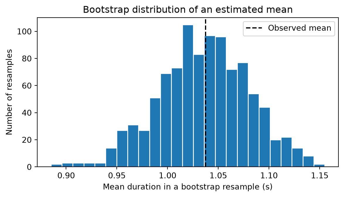
# Step 7: Start a separate reproducible bootstrap demonstration.import matplotlib.pyplot as plt# Use a fixed artificial sample, in seconds, rather than an external dataset.observed_sample_seconds = np.array([0.82, 0.91, 0.97, 1.02, 1.08, 1.13, 1.16, 1.21])# Reset a separate random stream so this demonstration does not depend on earlier draws.bootstrap_generator = np.random.default_rng(123)# One thousand resamples is a small teaching computation, not a universal accuracy setting.number_of_bootstrap_samples =1000# Store one estimated mean for each resample.bootstrap_means_seconds = np.empty(number_of_bootstrap_samples)# Step 8: Resample whole observations and recompute the statistic explicitly.for bootstrap_index inrange(number_of_bootstrap_samples):# Keep the resample size equal to the original sample size. resampled_durations = bootstrap_generator.choice( observed_sample_seconds, size=len(observed_sample_seconds), replace=True )# The statistic must be recomputed for each independently constructed resample. bootstrap_means_seconds[bootstrap_index] = np.mean(resampled_durations)# Step 9: Summarize the spread and central percentiles of the bootstrap distribution.# ddof=1 estimates the spread across the finite collection of bootstrap statistics.bootstrap_standard_error_seconds = np.std(bootstrap_means_seconds, ddof=1)# These are approximate percentile interval endpoints, not guaranteed 95% coverage.percentile_interval_seconds = np.quantile(bootstrap_means_seconds, [0.025, 0.975])print("Bootstrap estimated standard error (s):", bootstrap_standard_error_seconds)print("Approximate percentile interval (s):", percentile_interval_seconds)# Step 10: Display the distribution of estimates rather than raw durations.figure, axis = plt.subplots(figsize=(6.2, 3.6))axis.hist(bootstrap_means_seconds, bins=25, edgecolor="white")axis.axvline(np.mean(observed_sample_seconds), color="black", linestyle="--", label="Observed mean")axis.set_xlabel("Mean duration in a bootstrap resample (s)")axis.set_ylabel("Number of resamples")axis.set_title("Bootstrap distribution of an estimated mean")axis.legend()figure.tight_layout()plt.show()
Figure 8.1: Bootstrap distribution of the sample mean for artificial IID durations. The histogram describes resampled estimates, not individual-duration variability.
The histogram concerns estimated means, not the distribution of individual durations. Increasing \(B\) reduces Monte Carlo noise in the bootstrap calculation; it does not increase the eight original observations or remove their sampling limitations. When rows are dependent, resampling individual rows can seriously understate uncertainty. Subject-level or block resampling may be required, with the resampling unit matched to the scientific question.
8.9 Exercises and worked answers
Name the object. Is “average the next 20 measurements” an estimator or an estimate? Answer: an estimator, a rule before observing its numerical result. The resulting number is the estimate.
Separate SD and SE. IID observations have standard deviation 12 units. What is the mean’s standard error for \(n=36\)? Answer:\(12/\sqrt{36}=2\) units. The individual standard deviation remains 12; it is the mean that becomes less variable.
Check the variance denominator. Values \((2,4,6)\) have what unbiased sample variance? Answer: mean 4, squared deviations \(4,0,4\), and variance \(8/(3-1)=4\). The empirical variance is \(8/3\).
Interpret a confidence interval. Does a 95% mean interval contain 95% of future measurements? Answer: no. Its coverage concerns the fixed mean across repeated samples. Future individual measurements require a prediction interval.
Explain zero correlation. If \(Y=X^2\) and \(X\) has a symmetric distribution about zero, can dependence remain when covariance is zero? Answer: yes. \(Y\) is a deterministic function of \(X\); symmetry can make positive and negative products cancel in covariance.
Compare estimation criteria. Must maximum likelihood be unbiased? Answer: no. The normal variance maximum-likelihood estimate divides by \(n\), while unbiased sample variance divides by \(n-1\) under IID sampling.
Choose a bootstrap unit. A dataset has many windows from each of ten independent participants. Is row resampling automatically valid for participant-level uncertainty? Answer: no. Windows within a participant may be dependent. Resampling participants with their associated data may better match the target, though only ten independent participants still limits inference.
8.10 One-page revision summary
Concept
What to remember
Parameter / estimate
Unknown population quantity / observed numerical result.
Estimator / sampling distribution
Rule applied to data / variability of that rule across samples.
\(s^2\)
Divide centered squares by \(n-1\) for unbiased IID variance estimation.
Standard error
Spread of an estimator; for an IID mean, \(\sigma/\sqrt n\).
Covariance / correlation
Joint linear variation / its dimensionless standardization.
Normal likelihood
Equal-variance normal errors connect maximum likelihood with least squares.
Confidence interval
Coverage property of a procedure under assumptions.
Bootstrap
Resample appropriate independent units; more resamples are not more original data.
Check the population, observation unit, dependence, and sampling mechanism before interpreting a small standard error. The next two mathematics chapters, Chapter 9 and Chapter 10, explain how a fitting objective changes with its parameters and how a numerical procedure can seek its minimum.